Search for last-minute train slots (STDCM)

• 1: Business context
• 2: Train slot search module
• 2.1: Infrastructure exploration
• 2.2: Conflict detection
• 2.3: Conflict avoidance
• 2.4: Discontinuities and backtracking
• 2.5: Search space and decision tree
• 2.6: The actual pathfinding
• 2.7: Standard allowance
• 2.8: Implementation details and current issues

1 - Business context

Some definitions:

Capacity

Capacity, in this context, is the ability to reserve infrastructure elements to allow the passage of a train.

Capacity is expressed in both space and time: the reservation of an element can block a specific zone that becomes inaccessible to other trains, and this reservation lasts for a given time interval.

It can be displayed on a chart, with the time on the horizontal axis and the distance traveled on the vertical axis.

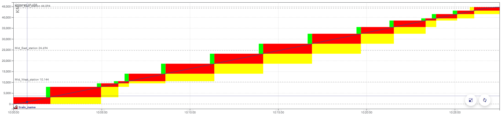
Example of a space-time chart displaying the passage of a train.

The colors here represent aspects of the signals, but display a consumption of the capacity as well: when these blocks overlap for two trains, they conflict.

There is a conflict between two trains when they reserve the same object at the same time, in incompatible configurations.

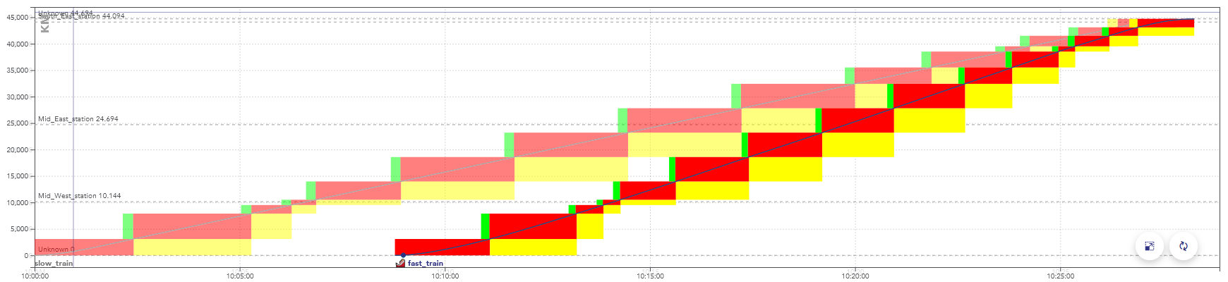
Example of a space-time graph with a conflict: the second train is faster than the first one, they are in conflict at the end of the path, when the rectangles overlap.

When simulating this timetable, the second train would be slowed down by the yellow signals, caused by the presence of the first train.

Train slots

A train slot corresponds to a capacity reservation for the passage of a train. It is fixed in space and time: the departure time and the path taken are known. On the space-time charts in this page, a train slot corresponds to the set of blocks displayed for a train.

Note: in English-speaking countries, these are often simply called “train paths”. But in this context, this name would be ambiguous with the physical path taken by the train.

The usual procedure is for the infrastructure manager (e.g. SNCF Réseau) to offers train slots for sale to railway companies (e.g. SNCF Voyageurs).

At a given date before the scheduled day of operation, all the train paths are allocated. But there may be enough capacity to fit more trains. Trains can fit between scheduled slots, when they are sufficiently far apart or have not found a buyer.

The remaining capacity after the allocation of train paths is called residual capacity. This section explains how OSRD looks for train slots in this residual capacity.

2 - Train slot search module

This module handles the search for solutions.

To summarize how it works: the search space is defined as one large decision tree.

We first build one decision tree that lists all possible paths, where each “decision” is the direction taken. We then build another tree on top of it that handles simulations and conflicts, branching is done when the new train gets to choose if it goes before or after a different train.

We then run an A* on the resulting graph.

2.1 - Infrastructure exploration

The first thing we need to define is how we move through the infrastructure, without dealing with conflicts yet.

We need a way to define and enumerate the different possible paths and explore the infrastructure graph, with several constraints:

1. The path must be compatible with the given rolling stock (loading gauge / electrification / signaling system)
2. At any point, we need to access path properties from its start up to the considered point. This includes block and route lists.
3. We sometimes need to know where the train will go after the point currently being evaluated, for proper conflict detection

To do this, we have defined the class InfraExplorer. It has one purpose: enumerating all possible paths. This is the class that handles the “path” aspect of the decision tree.

It uses blocks (sections from signal to signal) as a main subdivision. It has 3 sections: the current block, predecessors, and a “lookahead”.

In this example, the green arrows are the predecessor blocks. What happens there is considered to be immutable.

The red arrow is the current block. This is where we run train and signaling simulations, and where we deal with conflicts.

The blue arrows are part of the lookahead. This section hasn’t been simulated yet, its only purpose is to know in advance where the train will go next. In this example, it would tell us that the bottom right signal can be ignored entirely. The top path is the path being currently evaluated. The path that goes toward the bottom right track, if valid, will be evaluated in a different InfraExplorer that would have been generated alongside this instance.

The InfraExplorer is manipulated with two main functions (the accessors have been removed here for clarity):

interface InfraExplorer {
    /**
     * Clone the current object and extend the lookahead by one route, for each route starting at
     * the current end of the lookahead section. The current instance is not modified.
     */
    fun cloneAndExtendLookahead(): Collection<InfraExplorer>

    /**
     * Move the current block by one, following the lookahead section. Can only be called when the
     * lookahead isn't empty.
     */
    fun moveForward(): InfraExplorer
}

cloneAndExtendLookahead() is the method that actually enumerates the different paths, returning clones for each possibility. It’s called when we need a more precise lookahead to properly identify conflicts, or when it’s empty and we need to move forward.

A variation of this class can also keep track of the train simulation and time information (called InfraExplorerWithEnvelope). This is the version that is actually used to explore the infrastructure.

We now have a way to enumerate all possible paths:

2.2 - Conflict detection

Once we know what paths we can use, we need to know when they can actually be used.

The documentation of the conflict detection module explains how it’s done internally. Generally speaking, a train is in conflict when it has to slow down because of a signal. In our case, that means the solution would not be valid, we need to arrive later (or earlier) to see the signal when it’s not restrictive anymore.

In STDCM, conflicts can also be caused by work schedules.

The complex part is that we need to do the conflict detection incrementally Which means that:

1. When running simulations up to t=x, we need to know all of the conflicts that happen before x, even if they’re indirectly caused by a signal seen at t > x down the path.
2. We need to know the conflicts and resource uses right as they start even if their end time can’t be defined yet.

For that to be possible, we need to know where the train will go after the section that is being simulated (see infra exploration: we need some elements in the lookahead section).

To handle it, the conflict detection module returns an error when more lookahead is required. When it happens we extend it by cloning the infra explorer objects.

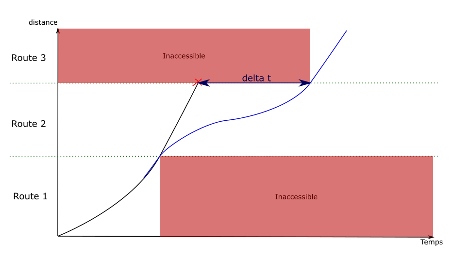
2.3 - Conflict avoidance

While exploring the graph, it is possible to end up in locations that would generate conflicts. They can be avoided by adding delay.

Shifting the departure time

The departure time is defined as an interval in the module parameters: the train can leave at a given time, or up to x seconds later. Whenever possible, delay should be added by shifting the departure time.

for example : a train can leave between 10:00 and 11:00. Leaving at 10:00 would cause a conflict, the train actually needs to enter the destination station 15 minutes later. Making the train leave at 10:15 solves the problem.

In OSRD, this feature is handled by keeping track, for every edge, of the maximum duration by which we can delay the departure time. As long as this value is enough, conflicts are avoided this way.

This time shift is a value stored in every edge of the path. Once a path is found, the value is summed over the whole path. This is added to the departure time.

For example :

• a train leaves between 10:00 and 11:00. The initial maximum time shift is 1:00.
• At some point, an edge becomes unavailable 20 minutes after the train passage. The value is now at 20 for any edge accessed from here.
• The departure time is then delayed by 5 minutes to avoid a conflict. The maximum time shift value is now at 15 minutes.
• This process is applied until the destination is found, or until no more delay can be added this way.

Engineering allowances

Once the maximum delay is at 0, the delay needs to be added between two points of the path.

The idea is the same as the one used to fix speed discontinuities: new edges are created, replacing the previous ones. The new edges have an engineering allowance, to add the delay where it is possible.

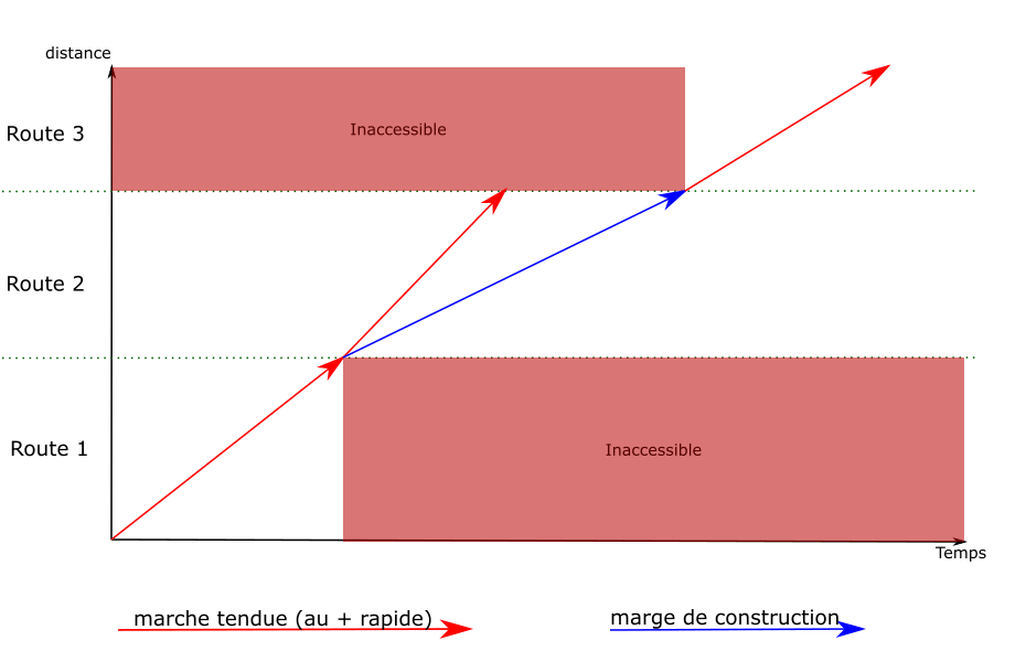
computing an engineering allowance is a feature of the running-time calculation module. It adds a given delay between two points of a path, without affecting the speeds on the rest of the path.

Post-processing

We used to compute the engineering allowances during the graph exploration, but that process was far too expensive. We used to run binary searches on full simulations, which would sometimes go back for a long distance in the path.

What we actually need is to know whether an engineering allowance is possible without causing any conflict. We can use heuristics here, as long as we’re on the conservative side: we can’t say that it’s possible if it isn’t, but missing solutions with extremely tight allowances isn’t a bad thing in our use cases.

But this change means that, once the solution is found, we can’t simply concatenate the simulation results. We need to run a full simulation, with actual engineering allowances, that avoid any conflict. This step has been merged with the one described on the standard allowance page, which is now run even when no standard allowance have been set.

2.4 - Discontinuities and backtracking

The discontinuity problem

When a new graph edge is visited, a simulation is run to evaluate its speed. But it is not possible to see beyond the current edge. This makes it difficult to compute braking curves, because they can span over several edges.

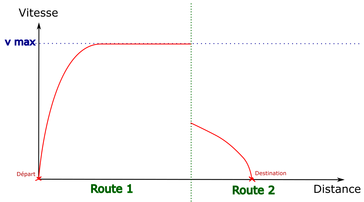
This example illustrates the problem: by default the first edge is explored by going at maximum speed. The destination is only visible once the second edge is visited, which doesn’t leave enough distance to stop.

Solution : backtracking

To solve this problem, when an edge is generated with a discontinuity in the speed envelopes, the algorithm goes back over the previous edges to create new ones that include the decelerations.

To give a simplified example, on a path of 4 edges where the train can accelerate or decelerate by 10km/h per edge:

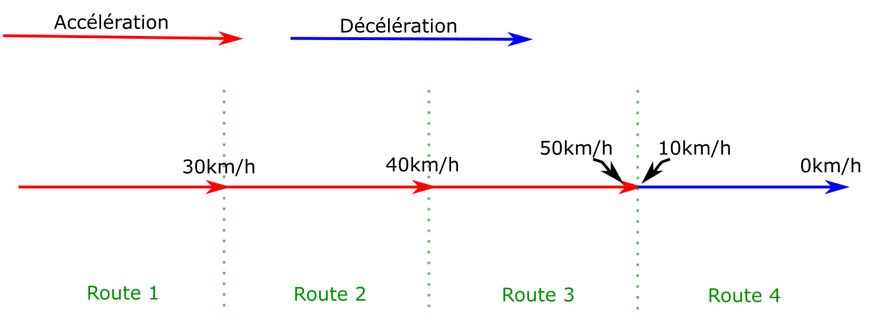
For the train to stop at the end of route 4, it must be at most at 10km/h at the end of edge 3. A new edge is then created on edge 3, which ends at 10km/h. A deceleration is computed backwards from the end of the edge back to the start, until the original curve is met (or the start of the edge).

In this example, the discontinuity has only been moved to the transition between edges 2 and 3. The process is then repeated on edge 2, which gives the following result:

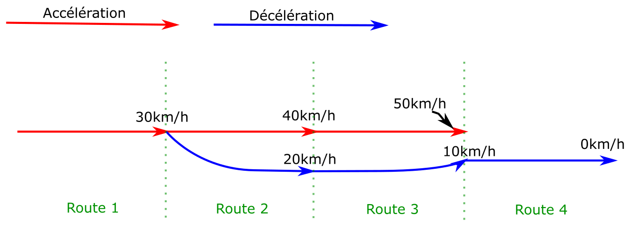
Old edges are still present in the graph as they can lead to other solutions.

2.5 - Search space and decision tree

Now that we can enumerate the paths and identify conflicts, we need to build the final decision tree that avoids all conflicts.

The search space is described as a graph with nodes and edges. Edges are generally one signaling block long, but may be shorter in case of stops.

Generating new edges on a given path follow this sequence:

1. The train movement is generated on the new segment (time and speed at each point)
2. Conflicts are identified during this time segment
3. Openings are identified
4. One edge is generated per opening

An “opening” is an available time window between two occupied blocks. When there are several different openings, we get to choose if the new train goes before or after another train or work schedule.

On one given path, we now have a decision tree that looks like this:

Delays

We often need to add delay to the current simulation to actually go through an opening, when the train needs to reach a point later than it could have.

This can be done in several different ways:

• Delaying the train departure
• Lengthening a stop
• Forcing the train to go slower for a while (with something called “engineering allowances”)

We keep track of how much delay we can add at any given point to handle departure and stop changes. For engineering allowances, we’re identifying how much delay we can add if the train slows down then immediately speeds up.

2.6 - The actual pathfinding

Once we have a graph that describes the entire search space, we can run a pathfinding algorithm. In this case, we use an A*.

We need to define a few things first:

• How to sort the nodes, which defines which solution is considered better than the other
• How to identify redundant nodes
• How to estimate the remaining “cost” at any given point (the heuristic)

Node ordering

We currently define a hierarchy across different criteria: we first compare the most important one, and move on to the next if equal, until we reach the end of the list.

That order is defined in STDCMNode, in compareTo. It tends to change more often than this website is updated, so it’s best to check the code itself.

The main criteria is the best possible total travel time: the sum of the current travel time to reach this node and the minimum remaining travel time from this node to the destination (as defined/computed by the heuristic). Stop duration isn’t included here.

Defining redundant (visited) nodes

This is handled by VisitedNodes.

The idea is that, at any given physical location, we mark time ranges as “visited”.

For example: consider a node reached at earliest t=10:00, where we can delay the departure by 30 minutes, and we can’t add any engineering allowance (added time by slowing down). Then the location will be flagged as “visited” from t=10:00 to t=10:30.

Engineering allowance means we can also reach some other time range by lengthening the travel time. But it may not be the optimal way to reach a given time. So we can mark a range as “conditionally visited”, where it’s visited at a given cost value. These ranges are compared to the new range and cost to identify if the new node is redundant.

Heuristic

Most of the algorithmic complexity here comes from the high number of nodes for any given location. Going through the entire block graph once is comparatively quite fast.

So we go through the entire block graph, starting at the destination, and we keep track of the fastest time it takes to reach the destination from any given point.

We keep track of intermediate path steps, max speed, and decelerations (including decelerations caused by requested stops). But we can’t consider accelerations at this stage.

It may sound slow and expensive (and it can be), but it drastically lowers the standard deviation and upper bound in search time.

2.7 - Standard allowance

The STDCM module must be usable with standard allowances. The user can set an allowance value, expressed either as a function of the running time or the travelled distance. This time must be added to the running time, so that it arrives later compared to its fastest possible running time.

For example: the user can set a margin of 5 minutes per 100km. On a 42km long path that would take 10 minutes at best, the train should arrive 12 minutes and 6 seconds after leaving.

This can cause problems to detect conflicts, as an allowance would move the end of the train slot to a later time. The allowance must be considered when we compute conflicts as the graph is explored.

The allowance should also follow the MARECO model: the extra time isn’t added evenly over the whole path, it is computed in a way that requires knowing the whole path. This is done to optimize the energy used by the train.

During the exploration

The main implication of the standard allowance is during the graph exploration, when we identify conflicts. It means that we need to scale down the speeds. We still need to compute the maximum speed simulations (as they define the extra time), but when identifying at which time we see a given signal, all speeds and times are scaled.

This process is not exact. It doesn’t properly account for the way the allowance is applied (especially for MARECO). But at this point we don’t need exact times, we just need to identify whether a solution would exist at this approximate time.

Post-processing

The process to find the actual train simulation is as follows:

1. We define points at which the time is fixed, initialized at first with the time of each train stop. This is an input of the simulation and indirectly calls the standard allowance.
2. We run a full simulation over the entire path with conflict detection
3. If there are conflicts, we try to remove the first one.
4. We add a fixed time point at the location where that conflict happened. We use the time considered during the exploration (with linear scaling) as reference time.
5. This process is repeated iteratively until no conflict is found.

This is the general idea. In practice, we need some workarounds to avoid some issues. These include:

• Adding a fixed time point at the end location of engineering allowances (when not part of a different engineering allowance)
• Distributing engineering allowance times linearly over the engineering allowance distance
• When we fail to find a valid solution, we fall back from MARECO to “linear” allowance distribution
• When we still fail to find a valid solution, we increase the train traction. This lets us find a close solution.

When we fail to find a solution despite all this, an error is thrown and needs to be investigated. It can be difficult to identify what went wrong though, it can come from any difference and mismatch between the search and this final post-processing simulation.

2.8 - Implementation details and current issues

This page is about implementation details. It isn’t necessary to understand general principles, but it helps before reading the code.

STDCMEdgeBuilder

This refers to this class in the project.

This class is used to make it easier to create instances of STDCMEdge, the graph edges. These contain many attributes, most of which can be determined from the context (e.g. the previous node). The STDCMEdgeBuilder class makes some parameters optional and automatically computes others.

Once instantiated and parameterized, an STDCMEdgeBuilder has two methods:

• makeAllEdges(): Collection<STDCMEdge> can be used to create all the possible edges in the given context for a given route. If there are several “openings” between occupancy blocks, one edge is instantiated for each opening. Every conflict, their avoidance, and their related attributes are handled here.

• findEdgeSameNextOccupancy(double timeNextOccupancy): STDCMEdge?: This method is used to get the specific edges that uses a certain opening (when it exists), identified here with the time of the next occupancy block. It is called whenever a new edge must be re-created to replace an old one. It calls the previous method.

Past path data

During the exploration, we simulate each block on its own, ignoring where the train comes from. This is done to improve caching, and because past path data is currently difficult to fetch.

This has two issues:

• We need to consider that speed limits apply until the train head leaves the speed limit range. This is technically wrong, it should be dismissed when the train tail leaves it.
• During the search, we don’t know the slopes on the tracks still covered by the train. This can lead to accelerations that are too optimistic, and in rare cases to post-processing errors.

There’s an open issue, but we don’t have a clear plan nor the time to work on it (yet).