Design documents are meant to help understand and participate in designing software.
Each design document describes a number of things about a piece of software:
- its goals
- its constraints
- how its inputs and outputs were modeled
- how it works
This is the multi-page printable view of this section. Click here to print.
Design documents are meant to help understand and participate in designing software.
Each design document describes a number of things about a piece of software:
Not translated: please select another language
The signaling layer includes all signals, which respond to track occupancy and reservation. Signals can be of different types, and are modularly loaded. Only their behavior towards the state of the infrastructure and the train’s reaction to signaling matters.
Signals are connected to each other by blocks. Blocks define paths permitted by signaling.
The signaling system is at the crossroads of many needs:
All static data:
To simulate signaling:
For speed limits:
Each signaling system has:
{
    # unique identifier for the signaling system
    "id": "BAL",
    "version": "1.0",
    # the schema of the dynamic state of signals of this type
    "signal_state": [
        {"kind": "enum", "field_name": "aspect", values: ["VL", "A", "S", "C"]},
        {"kind": "flag", "field_name": "ralen30"},
        {"kind": "flag", "field_name": "ralen60"},
        {"kind": "flag", "field_name": "ralen_rappel"}
    ],
    # describes static properties of the signal
    "signal_properties": [
        {"kind": "flag", "field_name": "Nf", "display_name": "Non-permissive"},
        {"kind": "flag", "field_name": "has_ralen30", "default": false, "display_name": "Ralen 30"},
        {"kind": "flag", "field_name": "has_rappel30", "default": false, "display_name": "Rappel 30"},
        {"kind": "flag", "field_name": "has_ralen60", "default": false, "display_name": "Ralen 60"},
        {"kind": "flag", "field_name": "has_rappel60", "default": false, "display_name": "Rappel 60"}
    ],
    # describes dynamic properties of the signal. These can be set on a per-route basis
    "signal_parameters": [
        {"kind": "flag", "field_name": "short_block", "default": false, "display_name": "Short block"},
        {"kind": "flag", "field_name": "rappel30", "default": false, "display_name": "Rappel 30"},
        {"kind": "flag", "field_name": "rappel60", "default": false, "display_name": "Rappel 60"}
    ],

    # these are C-like boolean expressions:
    # true, false, <flag>, <enum> == value, &&, || and ! can be used

    # used to evaluate whether a signal is a block boundary. Only properties can be used, not parameters.
    "block_boundary_when": "true",

    # used to evaluate whether a signal is a route boundary. Only properties can be used, not parameters.
    "route_boundary_when": "Nf",

    # A predicate used evaluate whether a signal state can make a train slow down. Used for naive conflict detection.
    "constraining_ma_when": "aspect != VL"
}
The blocks have several attributes:
The path is expressed from detector to detector so that it can be overlaid with the route graph.
A few remarks:
waypoints: List<DiDetector>signals: OrderedMap<Position, UnloadedSignal>speed_limits: RangeMap<Position, SpeedLimit>, including the logic for train category limitsPhysical signal are made up of one or more logical signals, which are displayed as a single unit on the field. During simulation, logical signals are treated as separate signals.
Each logical signal is associated with a signaling system, which defines if the signal transmits Movement Authority, speed limits, or both.
Logical signals have one or more drivers. Signal drivers are responsible for computing signal state. Any given signal driver only works for a given pair of signaling systems, where the first one is displayed by the signal, and the second is the one displayed by the next signal.
When a logical signal has an empty driver list, its content is deduced from neighboring signals.
For example, a BAL signal that is both a departure of the TVM block and a
departure of the BAL block, it will have two drivers: BAL-BAL and BAL-TVM.
When a signal announces a speed limit, it needs to be linked with a speed section object. This is meant to enable smooth transitions between the reaction to the announce signal, and the limit itself.
If multiple signals are involved in the announce process, only the one closest to the speed limit has to have this attribute set.
{
    # ...
    "announce_speed_section": "${SPEED_SECTION_ID}"
    # ...
}
Some signal parameters vary depending on which route is set. On each signal, an arbitrary number of rules can be added. If the signal is last to announce a speed limit, it must be explicitly mentioned in the rule.
{
    # ...
    "announce_speed_section": "${SPEED_SECTION_ID}",
    "default_parameters": {"short_block": "false"},
    "conditional_parameters": [
        {
            "on_route": "${ROUTE_ID}",
            "announce_speed_section": "${SPEED_SECTION_ID}",
            "parameters": {"rappel30": "true", "short_block": "true"}
        }
    ]
    # ...
}
Signal parameter values are looked up in the following order:
default_parameters).signal_parameters[].defaultThe serialized / raw format is the user-editable description of a physical signal.
Raw signals have a list of logical signals, which are independently simulated units sharing a common physical display. Each logical signal has:
For example, this signal encodes a BAL signal which:
{
    # signals must have location data.
    # this data is omitted as its format is irrelevant to how signals behave

    "logical_signals": [
        {
            # the signaling system shown by the signal
            "signaling_system": "BAL",
            # the settings for this signal, as defined in the signaling system manifest
            "properties": {"has_ralen30": "true", "Nf": "true"},
            # this signal can react to BAL or TVM signals
            # if the list is empty, the signal is assumed to be compatible with all following signaling systems
            "next_signaling_systems": ["BAL", "TVM"]
            "announce_speed_section": "${SPEED_SECTION_B}",
            "default_parameters": {"rappel30": "true", "short_block": "false"},
            "conditional_parameters": [
                {
                    "on_route": "${ROUTE_A}",
                    "announce_speed_section": "${SPEED_SECTION_C}",
                    "parameters": {"short_block": "true"}
                }
            ]
        }
    ]
}
For example, this signal encodes a BAL signal which starts a BAL block, and shares its physical display / support with a BAPR signal starting a BAPR block:
{
    # signals must have location data.
    # this data is omitted as its format is irrelevant to how signals behave

    "logical_signals": [
        {
            "signaling_system": "BAL",
            "properties": {"has_ralen30": "true", "Nf": "true"},
            "next_signaling_systems": ["BAL"]
        },
        {
            "signaling_system": "BAPR",
            "properties": {"Nf": "true", "distant": "false"},
            "next_signaling_systems": ["BAPR"]
        }
    ]
}
Signal definitions need to be condensed into a shorter form, just to look up signal icons. In order to store this into MVT map tiles hassle free, it’s condensed down into a single string.
It looks something like that: BAL[Nf=true,ralen30=true]+BAPR[Nf=true,distant=false]
It’s built as follows:
+,For signal state evaluation:
Railway infrastructure has a surprising variety of speed limits:
{
    # unique speed limit identifier
    "id": "...",

    # A list of routes the speed limit is enforced on. When empty
    # or missing, the speed limit is enforced regardless of the route.
    #
    # /!\ When a speed section is announced by signals, the routes it is
    # announced on are automatically filled in /!\
    "on_routes": ["${ROUTE_A}", "${ROUTE_B}"]
    # "on_routes": null, # not conditional
    # "on_routes": [], # conditional

    # A speed limit in meters per second.
    "speed_limit": 30,

    # A map from train tag to speed limit override. If missing and
    # the speed limit is announced by a signal, this field is deduced
    # from the signal.
    "speed_limit_by_tag": {"freight": 20},

    "track_ranges": [{"track": "${TRACK_SECTION}", "begin": 0, "end": 42, "applicable_directions": "START_TO_STOP"}],
}
When a speed limit is announced by dynamic signaling, we may be in a position where speed limit value is duplicated:
There are multiple ways this issue can be dealt with:
Upsides:
Downsides:
This option was not explored much, as it was deemed awkward to deduce signal parameters from a speed limit value.
Make the speed limit value optional, and deduce it from the signal itself. Speed limits per tag also have to be deduced if missing.
Upsides:
Downsides:
Speed limit announced by dynamic signaling often start being enforced at a specific location, which is distinct from the signal which announces the speed limit.
To allow for correct train reactions to this kind of limits, a link between the announce signal and the speed limit section has to be made at some point.
Was not deemed realistic.
Was deemed to be awkward, as signaling is currently built over interlocking. Referencing signaling from interlocking creates a circular dependency between the two schemas.
Add a list of (route, signal) tuples to speed sections.
Upside:
Downside:
Introduces a new type of speed limit, which are announced by signals. These speed limits are directly defined within signal definitions.
{
    # ...
    "conditional_parameters": [
        {
            "on_route": "${ROUTE_ID}",
            "speed_section": {
                "speed_limit": 42,
                "begin": {"track": "a", "offset": 10},
                "end": {"track": "b", "offset": 15},
            },
            "parameters": {"rappel30": "true", "short_block": "true"}
        }
    ]
    # ...
}
Upsides:
Downsides:
{
    # ...
    "conditional_parameters": [
        {
            "on_route": "${ROUTE_ID}",
            "announced_speed_section": "${SPEED_SECTION_ID}",
            "parameters": {"rappel30": "true", "short_block": "true"}
        }
    ]
    # ...
}
Upsides:
Downsides:
Some speed limits only apply so some routes. This relationship needs to be modeled:
We took option 3.
The first step of loading the signal is to characterize the signal in the signaling system. This step produces an object that describes the signal.
During the loading of the signal:
Once signal parameters are loaded, drivers can be loaded. For each driver:
(signaling_system, next_signaling_system) pair.This step produces a Map<SignalingSystem, SignalDriver>, where the signaling
system is the one incoming to the signal. It then becomes possible to construct
the loaded signal.
The validation process helps to report invalid configurations in terms of signaling and blockage. The validation cases we want to support are:
In practice, there are two separate mechanisms to address these two needs:
extern fn report_warning(/* TODO */);
extern fn report_error(/* TODO */);

struct Block {
   startsAtBufferStop: bool,
   stopsAtBufferStop: bool,
   signalTypes: Vec<SignalingSystemId>,
   signalSettings: Vec<SignalSettings>,
   signalPositions: Vec<Distance>,
   length: Distance,
}

/// Runs in the signaling system module
fn check_block(
   block: Block,
);


/// Runs in the signal driver module
fn check_signal(
   signal: SignalSettings,
   block: Block, // The partial block downstream of the signal - no signal can see backward
);
Before a train startup:
During the simulation:
Signals are modeled as an evaluation function, taking a view of the world and returning the signal state
enum ZoneStatus {
   /** The zone is clear to be used by the train */
   CLEAR,
   /** The zone is occupied by another train, but otherwise clear to use */
   OCCUPIED,
   /** The zone is incompatible. There may be another train as well */
   INCOMPATIBLE,
}

interface MAView {
    /** Combined status of the zones protected by the current signal */
    val protectedZoneStatus: ZoneStatus
    val nextSignalState: SignalState
    val nextSignalSettings: SignalSettings
}

fun signal(maView: MAView?): SignalState {
    // ...
}
The view should allow access to the following data:
The path along which the MAView and SpeedLimitView live is best expressed using blocks:
Everything mentioned so far was designed to simulate signals between a train the end of its movement authority, as all others signals have no influence over the behavior of trains (they cannot be seen, or are disregarded by drivers).
Nevertheless, one may want to simulate and display the state of all signals at a given point in time, regardless of which signals are in use.
Simulation rules are as follows:
This document is a work in progress
Conflict detection is the process of looking for timetable conflicts. A timetable conflict is any predictable condition which disrupts planned operations. Planned operations can be disrupted if a train is slowed down, prevented from proceeding, or delayed.
One of the core features of OSRD is the ability to automatically detect some conflicts:
Some other kinds of conflicts may be detected later on:
Conflict detection relies on interlocking and signaling modeling and simulation to:
The primary design goals are as follows:
In addition to these goals, the following constraints apply:
Actors are objects which cause resources to be used:
Actors need resources to be available to proceed, such as:
Actor emit resource requirements, which:
Resource requirements can turn out to be either satisfied or conflicting with other requirements, depending on compatibility rules.
Compatibility rules differ by requirement purpose and resource type. For example:
For conflict detection to work, resource requirements have to be at least as extensive as what’s required to guarantee that a train path will not be disturbed.
For trains to proceed safely along their planned path:
In practice, the path of trains is partitioned into routes, which when set, ensure a train can safely follow the route.
Routes have the following lifestyle:
For a train to proceed through a route unimpeded, the following things have to happen:
struct RouteRequirement {
    route: RouteId,
    set_deadline: Time,
    zone_requirements: Vec<RouteZoneRequirement>,
}

struct RouteZoneRequirement {
    zone: ZoneId,
    entry_det: DirDetectorId,
    exit_det: DirDetectorId,
    release_time: Time,
    switches: Map<SwitchId, SwitchConfigId>,
}
Routing requirements are generated by the following algorithm:
Route overlaps are not yet supported.
Requirement compatibility is evaluated for all RouteZoneRequirements, grouped by zone. Requirements A and B, ordered such that A.set_deadline <= B.set_deadline, are compatible if and only if either:
A.release_time <= (B.set_deadline - activation_time), where the activation time is the delay required to reconfigure from A.switches to B.switches.(A.entry_det, A.exit_det, A.switches) == (B.entry_det, B.exit_det, B.switches)Even if interlocking mitigates some of the risks associated with operating trains, a major one is left out: head to tail collisions, caused by insufficient spacing.
This responsibility is handled by signaling, which conveys both interlocking and spacing constraints.
Signaling helps trains slow down until the end of their movement authority, which is either:
Spacing requirements are emitted for zones which if occupied, would cause a slowdown, and zones occupied by the train
struct SpacingRequirement {
    zone: ZoneId,
    begin_time: Time,
    end_time: Time,
}
Every time the driver sees a signal, generate updated spacing requirements by calculating which zones, if occupied, would trigger a slowdown:
Requirement compatibility is evaluated for all SpacingRequirements, grouped by zone.
Requirements A and B are compatible if and only if their [begin_time, end_time] ranges do not overlap.
sequenceDiagram
    participant client as Client
    participant gen as Routing resource generator
    client ->> gen: initial path + train movement
    loop
        gen ->> client: prefix path extension needed
        client ->> gen: extra prefix path + train movement
    end
    gen ->> client: resource requirements
After an initial path is given, the requirement generator can ask for more prefix path (before the start of the route). The client responds with:
If the initial path has multiple routes, the last route is the one resource requirements are emitted for.
sequenceDiagram
    participant client as Client
    participant gen as Spacing resource generator
    client ->> gen: initial path + train movement
    loop
        gen ->> client: postfix path extension needed
        client ->> gen: extra postfix path
    end
    gen ->> client: resource requirements
After an initial path is given, the requirement generator can ask for more postfix path (before the start of the route).
This work is pending implementation, and has not yet been adjusted to reflect potential required adjustments.
These articles describe the design of the new train simulation system.
This system should be simpler and more stable than the current one, and should enable more advanced features in the future.
This work is pending implementation, and has not yet been adjusted to reflect potential required adjustments.
After two years of extending a fairly simple simulation engine, it appeared that fundamental changes are required to meet expectations.
The new system is expected to:
In the long-term, this system is also expected to:
flowchart TD
subgraph Input
    InitTrainState[initial train state]
    PathPhysicsProps[path physics properties]
    AbstractDrivingInstructions[abstract driving instructions]
    TargetSchedule[target schedule]
end

DrivingInstructionCompiler([driving instruction compiler])
ConcreteDrivingInstructions[driving instructions + limits]
ScheduleController([schedule controller])
DriverBehaviorModule([driver behavior module])

TargetSchedule --> ScheduleController
ScheduleController -- adjusts slowdown coefficient --> DriverBehaviorModule
AbstractDrivingInstructions --> DrivingInstructionCompiler
PathPhysicsProps --> DrivingInstructionCompiler
ScheduleController -- tracks train state --> TrainSim

DriverBehaviorModule -- makes decisions --> TrainSim
ConcreteDrivingInstructions --> DriverBehaviorModule
DrivingInstructionCompiler --> ConcreteDrivingInstructions

InitTrainState --> ScheduleController

TrainSim --> SimResults

TrainSim([train simulator])
SimResults[simulation result curve]The target schedule is a list of target arrival times at points specified along the path. To respect the schedule, the train may have to not use its maximum traction.
The train state is a vector of properties describing the train at a given point in time.
Driving instructions model what the train has to do along its path. They are linked to conditions on their application, and can interact with each other. They are generated using domain constraints such as speed limits or stops.
See the dedicated page for more details.
Path properties are the physical properties of the path, namely elevation, curves and electrification.
The driver behavior modules update the train state based on:
The train state changes should be physically realistic.
See the dedicated page for more details.
The schedule controller manages the slowdown coefficient given to the driver behavior module in order to respect the target schedule.
It adjusts the slowdown coefficient iteratively, using a dichotomous search, re-simulating the train behavior between two time-targeted points.
The output of the simulation is the list of train states at each time step.
The main idea of the new train simulator is to have a simulation which is computed step by step and not post-processed. This would ensure the physical consistency of the simulation.
The challenge is then to add ways to lose some time, in order to respect the target schedule.
This is done by iterating over the sections between two scheduled points, while adjusting a slowdown factor.
This slowdown factor would be used to control how the driver behavior module would lose time while still being
physically realistic.
See the driver behavior module dedicated page for more details.
In order to accommodate an infrastructure which could change with time (like signals), we introduce driving instructions.
These instructions are generated from the path properties and the target schedule, and are used to update the train state.
Instructions can be conditional, and can interact with each other.
The algorithm is described in detail in the dedicated page.

The current implementation has a number of shortcomings making it pretty much impossible to evolve to meet current system requirements. It also has a number of less severe flaws, such as the over-reliance on floating point, especially for input and output.
The previous implementation cannot be changed to:
These limitations are the primary reasons for this redesign.
are defined as post-processing filter passes on simulation results. This has a number of undesirable side effects:
margin algorithms produce the final simulation results. They may produce physically unrealistic simulations results
because margins are applied after the simulation, the simulation can’t adjust to impossible margin values. Thus the simulation fails instead of giving a “best effort” result.
margin algorithms have no choice but to piece together results of different simulations:
how much time should be lost and where isn’t defined in a way that makes scheduled points implementation easy
when a transition between two margin values occurs, slow downs occur before value changes, and speed ups after value changes. This is nice in theory, because it makes the graphs look nicer. The downside is that it makes margin values interdependent at each slow-down, as how much speed needs to be lost affects the time lost in the section.
With the previous implementation, the simulation takes sequence of constraint position and speed curves as an input (continuous in position, can be discontinuous in speed), and produces a continuous curve.
The output is fine, but the input is troublesome:
Driving instructions model what the train has to do, and under what conditions. Driving instructions are generated using domain constraints such as:
There are two types of driving instructions:
flowchart TD
Constraint[constraint]
AbstractDrivingInstruction[abstract driving instruction]
ConcreteDrivingInstruction[concrete driving instruction]
RollingStockIntegrator[rolling stock integrator]
Compiler([compiler])

Constraint -- generates one or more --> AbstractDrivingInstruction
AbstractDrivingInstruction --> Compiler
RollingStockIntegrator --> Compiler
Compiler --> ConcreteDrivingInstruction
After reviewing the design document, the necessity to distinguish between abstract and concrete driving instructions was questioned.
Indeed, it isn’t clear whether the limit curves are used for the driving instructions interpretation algorithm. If it isn’t, the computation of limit curves could be moved inside the driver behavior module.
TODO: remove this message or fix the design document after implementation.
During the simulation, driving instructions are partitioned into 4 sets:
PENDING instructions may apply at some point in the futureRECEIVED instructions aren’t enforced yet, but will be unless overriddenENFORCED instructions influence train behaviorDISABLED instructions don’t ever have to be considered anymore. There are multiple ways instructions can be disabled:SKIPPED instructions were not receivedRETIRED instructions expired by themselvesOVERRIDDEN instructions were removed by another instructionflowchart TD
subgraph disabled
skipped
retired
overridden
end
subgraph active
received
enforced
end
pending --> received
pending --> skipped
received --> enforced
received --> overridden
enforced --> retired
enforced --> overriddenThese sets evolve as follows:
PENDING instruction’s received condition, it is RECEIVED and becomes a candidate to executionOVERRIDDEN due to an override_on_received operationSKIPPED stateENFORCED. Only enforced instructions influence train behavior.OVERRIDDEN due to an override_on_enforced operationRETIREDWhen an instruction transitions to the RECEIVED or ENFORCED state, it can disable active instructions
which match some metadata predicate. There are two metadata attributes which can be relied on for overrides:
kind allows overriding previous instructions for a given domain, such as spacing or block signaled speed limitsrank can be used as a “freshness” or “priority” field. If two instructions overriding each other are received
(such as when a train sees two signals), the rank allows deciding which instruction should be prioritized.This is required to implement a number of signaling features, as well as stops, where the stop instruction is overridden by the restart instruction.
struct ReceivedCond {
    position_in: Option<PosRange>,
    time_in: Option<TimeRange>,
}

struct InstructionMetadata {
    // state transitions
    received_when: ReceivedCond,
    enforced_at: Position,
    retired_at: Option<Position>,

    // instruction metadata, used by override filters. if an instruction
    // has no metadata nor retiring condition, it cannot be overridden.
    kind: Option<InstructionKindId>,  // could be SPACING, SPEED_LIMIT
    rank: Option<usize>,

    // when the instruction transitions to a given state,
    // instructions matching any filter are overridden
    override_on_received: Vec<OverrideFilter>,
    override_on_enforced: Vec<OverrideFilter>,
}

enum AbstractInstruction {
    NeutralZone,
    SpeedTarget {
        at: Position,
        speed: Speed,
    }
}

enum ConcreteInstruction {
    NeutralZone,
    SpeedTarget {
        braking_curve: SpeedPosCurve,
    },
}

struct OverrideFilter {
    kind: InstructionKindId,
    rank: Option<(RankRelation, usize)>,
}

enum RankRelation {
    LT, LE, EQ, GE, GT
}
Early on, we started making lists of what domain constraints can have an impact on train behavior. Meanwhile, to simulate train behavior, we figured out that we need to know which constraints apply at any given time.
There’s a fundamental tension between these two design constraints, which can be resolved in one of two ways:
When we first started drafting architecture diagrams, the train simulation API directly took a bunch of constraint types as an input. It brought up a number of issues:
We couldn’t find clear benefits to dragging distinctions between constraint types deep into the implementation.
We then realized that abstracting over constraint types during simulation had immense benefits:
We decided to explore the possibility of keeping constraint types distinct in the external API, but lowering these constraints into an intermediary representation internally. We found a number of downsides:
We tried to improve over the previous proposal by moving the burden of converting many constraints into a common abstraction out of the simulation API.
Instead of having many constraint types as an input, the simulation API takes a collection of a single abstract constraint type. The task of converting domain constraints to abstract driving instructions is left to the API user.
We found that doing so:
As the train progresses through the simulation, it reacts according to driving instructions which depend on more than the bare train physics state (position, time, and speed):
Thus, given:
There is a need to know what driving instructions are applicable to the current integration step.
Overrides are a way of modeling instructions which disable previous ones. Here are some examples:
We identified multiple filtering needs:
We quickly settled on adding a kind field, but had a lengthy discussion over how to discriminate upstream and downstream signals. We explored the following options:
source metadata, which was rejected as it does not address the issue of upstream / downstreamDriver behavior modules are responsible for making driving decisions. Its main responsibility, given the state of the train and an instruction, is to react to the instruction. This reaction is expressed as a new train state.
To perform this critical task, it needs access to additional context:
The driver behavior modules are supposed to have different implementations, which would interpret the slow down coefficient differently.
One driver behavior module is instantiated per driving instruction. It takes at initialization:
It has two public methods:
enact_decision(current_state: TrainState, t: float) -> (TrainState, float)
Which returns what the next train state would be if there was only this one instruction to follow, and the time delta to reach this state.
truncate_integration_step(current_state: TrainState, potential_state: TrainState, t: float, dt: float) -> (TrainState, float)
Which returns a state and time delta which respects the instruction, and is as close as possible to the potential state.
At a given train state, we know which driving instructions are enforced.
For each enforced driving instruction, we query the corresponding driver behavior module.
This gives a set of different train states. From this, we coalesce a single train state which respects all instructions.
To do so, we:
dt they are associated with.truncate_integration_step.There is a heavy underlying assumption that “constraining properties” can be combined in a new state which is valid. This underlies the step 3. It is not yet clear if this assumption will always be valid in the future.
Also: what component should be in charge of instantiating all the driver behavior modules with the right implementation ?
Here is a schema summarizing the process:


Here the constraints are in red, and the next state chosen by the driver behavior modules are in black.
In this example, the most constraining state is A, since it’s the one which accelerates the least. However, it overshoots constraint B, thus we need to select the state which respects both constraints.
When this design project started, driver behavior was left completely undefined. We assumed that a set of driving instructions can be unambiguously interpreted given a starting point. This assumption was then decided to be relied on to search which margin speed ceiling yields expected arrival times.
We also knew this assumption to be false: there are many ways instructions can be interpreted. Worse yet, different use cases for OSRD have different needs:
To resolve this tension, we thought of adding support for pluggable driver behavior. Doing so, however, would create two ways a timetable can be loosened (loose time):
Let’s say we want to loosen the timetable by 1 minute on a given section. It could be achieved by:
This is an issue, as it might make simulation results unstable: because there possibly are many ways to achieve the requested schedule, it would be very challenging to reliably choose a solution which matches expectations.
Driver behavior can be formally modeled as a local decision function f, which takes the state of the
train as an input, including position and speed, and returns an acceleration.
To best integrate this acceleration over the given time step, it is best not to use only the acceleration at (t).
Since it may vary a lot along [t, t+dt]. To approximate the acceleration within this interval,
we would need a better estimator, using a numerical method such as
RK4. Such estimator then needs to call f multiple times.
A number of questions came up:
We identified that this API choice shouldn’t constrain the implementation. We decided to go the conservative route and have one DBM per driving instructions as it reduces the API surface and relieves DBM from the responsibility of finding the most restrictive instruction.
We identified that DBMs need the ability to follow internal target curves (distinct from limit curves).
To do so we could either:
We decided that only the first option was desirable.
The design choices then are:
Then the DBM would not be aware of the time step it is called with, and would return an acceleration. Then the module should expose two methods:
One for taking decisions, akin to f.
Called several times depending on the integration method.
One for correcting an integration step (i.e. a time step and a new state), if it happened to overshoot its internal goal curves
(for example MARECO which sets it’s own speed limits).
Called on the integration step results from this DBM, and the other DBMs integration step results.
The module would then expose two methods:
One for taking decisions, which, given a train state and a desired/maximum time step, returns a new state (which does not overshoot) and a new current time.
One for correcting an integration step (i.e. a time step and a new state), if it happened to overshoot its internal goal curves
(for example MARECO which sets it’s own speed limits).
Called only on other DBMs integration step results.
dt.dt amongst constraining properties. Interpolate remaining properties to this dt, to build a provisional state.dt.To understand how this algorithm is designed, we need to consider two example cases:
dt for the overshot constraint.truncate_integration_step depend on the driver behavior module?Yes: DBMs may use internal representations that the new state should not overshoot. For instance, when passed a driving instruction with a speed limit of 60km/h, a DBM wishing to lose time may reduce the speed to 50 km/h.
OSRD can be used to find a slot for a train in an already established timetable, without causing conflicts with other trains.
The acronym STDCM (Short Term Digital Capacity Management) is used to describe this concept in general. It’s sometimes called LMR (“last minute request”) when talking about the actual product in SNCF.
For video explanations, the subject has been explained twice at FOSDEM with replays available: in 2023 and in 2026. The first video focuses on the technical details, it’s quite old and thus incomplete, but only a few details are actually wrong. The second video does a quick explanation of the implementation, but focuses more on how it’s integrated in SNCF processes.
Some definitions:
Capacity, in this context, is the ability to reserve infrastructure elements to allow the passage of a train.
Capacity is expressed in both space and time: the reservation of an element can block a specific zone that becomes inaccessible to other trains, and this reservation lasts for a given time interval.
It can be displayed on a chart, with the time on the horizontal axis and the distance traveled on the vertical axis.
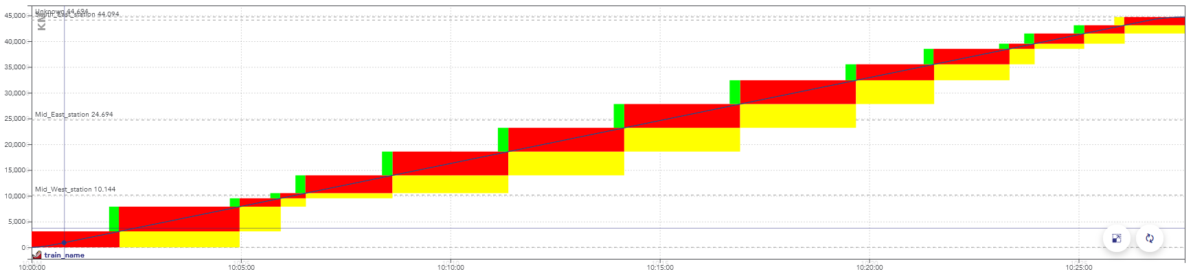
Example of a space-time chart displaying the passage of a train.
The colors here represent aspects of the signals, but display a consumption of the capacity as well: when these blocks overlap for two trains, they conflict.
There is a conflict between two trains when they reserve the same object at the same time, in incompatible configurations.
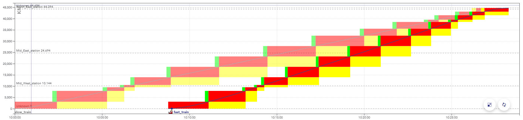
Example of a space-time graph with a conflict: the second train is faster than the first one, they are in conflict at the end of the path, when the rectangles overlap.
When simulating this timetable, the second train would be slowed down by the yellow signals, caused by the presence of the first train.
A train slot corresponds to a capacity reservation for the passage of a train. It is fixed in space and time: the departure time and the path taken are known. On the space-time charts in this page, a train slot corresponds to the set of blocks displayed for a train.
Note: in English-speaking countries, these are often simply called “train paths”. But in this context, this name would be ambiguous with the physical path taken by the train.
The usual procedure is for the infrastructure manager (e.g. SNCF Réseau) to offers train slots for sale to railway companies (e.g. SNCF Voyageurs).
At a given date before the scheduled day of operation, all the train paths are allocated. But there may be enough capacity to fit more trains. Trains can fit between scheduled slots, when they are sufficiently far apart or have not found a buyer.
The remaining capacity after the allocation of train paths is called residual capacity. This section explains how OSRD looks for train slots in this residual capacity.
This module handles the search for solutions.
To summarize how it works: the search space is defined as one large decision tree.
We first build one decision tree that lists all possible paths, where each “decision” is the direction taken. We then build another tree on top of it that handles simulations and conflicts, branching is done when the new train gets to choose if it goes before or after a different train.
We then run an A* on the resulting graph.
The first thing we need to define is how we move through the infrastructure, without dealing with conflicts yet.
We need a way to define and enumerate the different possible paths and explore the infrastructure graph, with several constraints:
To do this, we have defined the class InfraExplorer.
It has one purpose: enumerating all possible paths.
This is the class that handles the “path” aspect of the decision tree.
It uses blocks (sections from signal to signal) as a main subdivision. It has 3 sections: the current block, predecessors, and a “lookahead”.

In this example, the green arrows are the predecessor blocks. What happens there is considered to be immutable.
The red arrow is the current block. This is where we run train and signaling simulations, and where we deal with conflicts.
The blue arrows are part of the lookahead. This section hasn’t
been simulated yet, its only purpose is to know in advance
where the train will go next. In this example, it would tell us
that the bottom right signal can be ignored entirely.
The top path is the path being currently evaluated.
The path that goes toward the bottom right track, if valid,
will be evaluated in a different InfraExplorer that would have
been generated alongside this instance.
The InfraExplorer is manipulated with two main functions
(the accessors have been removed here for clarity):
interface InfraExplorer {
    /**
     * Clone the current object and extend the lookahead by one route, for each route starting at
     * the current end of the lookahead section. The current instance is not modified.
     */
    fun cloneAndExtendLookahead(): Collection<InfraExplorer>

    /**
     * Move the current block by one, following the lookahead section. Can only be called when the
     * lookahead isn't empty.
     */
    fun moveForward(): InfraExplorer
}
cloneAndExtendLookahead() is the method that actually enumerates the
different paths, returning clones for each possibility.
It’s called when we need a more precise lookahead to properly identify
conflicts, or when it’s empty and we need to move forward.
A variation of this class can also keep track of the train simulation
and time information (called InfraExplorerWithEnvelope).
This is the version that is actually used to explore the infrastructure.
We now have a way to enumerate all possible paths:

Once we know what paths we can use, we need to know when they can actually be used.
The documentation of the conflict detection module explains how it’s done internally. Generally speaking, a train is in conflict when it has to slow down because of a signal. In our case, that means the solution would not be valid, we need to arrive later (or earlier) to see the signal when it’s not restrictive anymore.
In STDCM, conflicts can also be caused by work schedules.
The complex part is that we need to do the conflict detection incrementally Which means that:
For that to be possible, we need to know where the train will go after the section that is being simulated (see infra exploration: we need some elements in the lookahead section).
To handle it, the conflict detection module returns an error when more lookahead is required. When it happens we extend it by cloning the infra explorer objects.
IncrementalConflictDetector. When debugging in local,
it can be inspected and patched to identify exactly where requirements come from.While exploring the graph, it is possible to end up in locations that would generate conflicts. They can be avoided by adding delay.
The departure time is defined as an interval in the module parameters:
the train can leave at a given time, or up to x seconds later.
Whenever possible, delay should be added by shifting the departure time.
for example : a train can leave between 10:00 and 11:00. Leaving at 10:00 would cause a conflict, the train actually needs to enter the destination station 15 minutes later. Making the train leave at 10:15 solves the problem.
In OSRD, this feature is handled by keeping track, for every edge, of the maximum duration by which we can delay the departure time. As long as this value is enough, conflicts are avoided this way.
This time shift is a value stored in every edge of the path. Once a path is found, the value is summed over the whole path. This is added to the departure time.
For example :
- a train leaves between 10:00 and 11:00. The initial maximum time shift is 1:00.
- At some point, an edge becomes unavailable 20 minutes after the train passage. The value is now at 20 for any edge accessed from here.
- The departure time is then delayed by 5 minutes to avoid a conflict. The maximum time shift value is now at 15 minutes.
- This process is applied until the destination is found, or until no more delay can be added this way.
Once the maximum delay is at 0, the delay needs to be added between two points of the path.
The idea is the same as the one used to fix speed discontinuities: new edges are created, replacing the previous ones. The new edges have an engineering allowance, to add the delay where it is possible.
computing an engineering allowance is a feature of the running-time calculation module. It adds a given delay between two points of a path, without affecting the speeds on the rest of the path.
We used to compute the engineering allowances during the graph exploration, but that process was far too expensive. We used to run binary searches on full simulations, which would sometimes go back for a long distance in the path.
What we actually need is to know whether an engineering allowance is possible without causing any conflict. We can use heuristics here, as long as we’re on the conservative side: we can’t say that it’s possible if it isn’t, but missing solutions with extremely tight allowances isn’t a bad thing in our use cases.
But this change means that, once the solution is found, we can’t simply concatenate the simulation results. We need to run a full simulation, with actual engineering allowances, that avoid any conflict. This step has been merged with the one described on the standard allowance page, which is now run even when no standard allowance have been set.
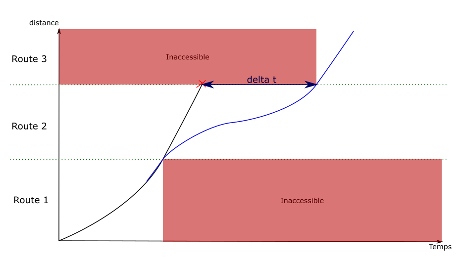
When a new graph edge is visited, a simulation is run to evaluate its speed. But it is not possible to see beyond the current edge. This makes it difficult to compute braking curves, because they can span over several edges.
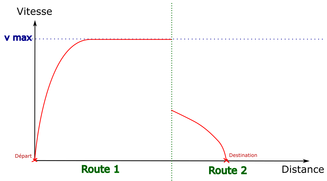
This example illustrates the problem: by default the first edge is explored by going at maximum speed. The destination is only visible once the second edge is visited, which doesn’t leave enough distance to stop.
To solve this problem, when an edge is generated with a discontinuity in the speed envelopes, the algorithm goes back over the previous edges to create new ones that include the decelerations.
To give a simplified example, on a path of 4 edges where the train can accelerate or decelerate by 10km/h per edge:
![]()
For the train to stop at the end of route 4, it must be at most at 10km/h at the end of edge 3. A new edge is then created on edge 3, which ends at 10km/h. A deceleration is computed backwards from the end of the edge back to the start, until the original curve is met (or the start of the edge).
In this example, the discontinuity has only been moved to the transition between edges 2 and 3. The process is then repeated on edge 2, which gives the following result:
![]()
Old edges are still present in the graph as they can lead to other solutions.
Now that we can enumerate the paths and identify conflicts, we need to build the final decision tree that avoids all conflicts.
InfraExplorer, but currently it’s all over the place.
There’s a refactoring issue,
but we may not have the time to do it.The search space is described as a graph with nodes and edges. Edges are generally one signaling block long, but may be shorter in case of stops.
Generating new edges on a given path follow this sequence:
An “opening” is an available time window between two occupied blocks. When there are several different openings, we get to choose if the new train goes before or after another train or work schedule.
On one given path, we now have a decision tree that looks like this:

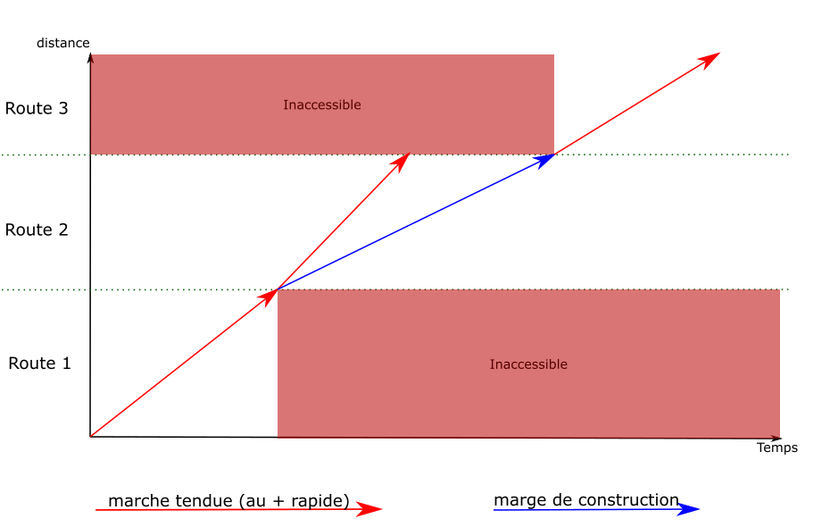
We often need to add delay to the current simulation to actually go through an opening, when the train needs to reach a point later than it could have.
This can be done in several different ways:
We keep track of how much delay we can add at any given point to handle departure and stop changes. For engineering allowances, we’re identifying how much delay we can add if the train slows down then immediately speeds up.
Once we have a graph that describes the entire search space, we can run a pathfinding algorithm. In this case, we use an A*.
We need to define a few things first:
We currently define a hierarchy across different criteria: we first compare the most important one, and move on to the next if equal, until we reach the end of the list.
That order is defined in STDCMNode,
in compareTo. It tends to change more often than this website
is updated, so it’s best to check the code itself.
The main criteria is the best possible total travel time: the sum of the current travel time to reach this node and the minimum remaining travel time from this node to the destination (as defined/computed by the heuristic). Stop duration isn’t included here.
This is handled by VisitedNodes.
The idea is that, at any given physical location, we mark time ranges as “visited”.
For example: consider a node reached at earliest t=10:00, where we can delay the departure by 30 minutes, and we can’t add any engineering allowance (added time by slowing down). Then the location will be flagged as “visited” from t=10:00 to t=10:30.
Engineering allowance means we can also reach some other time range by lengthening the travel time. But it may not be the optimal way to reach a given time. So we can mark a range as “conditionally visited”, where it’s visited at a given cost value. These ranges are compared to the new range and cost to identify if the new node is redundant.
Most of the algorithmic complexity here comes from the high number of nodes for any given location. Going through the entire block graph once is comparatively quite fast.
So we go through the entire block graph, starting at the destination, and we keep track of the fastest time it takes to reach the destination from any given point.
We keep track of intermediate path steps, max speed, and decelerations (including decelerations caused by requested stops). But we can’t consider accelerations at this stage.
It may sound slow and expensive (and it can be), but it drastically lowers the standard deviation and upper bound in search time.
The STDCM module must be usable with standard allowances. The user can set an allowance value, expressed either as a function of the running time or the travelled distance. This time must be added to the running time, so that it arrives later compared to its fastest possible running time.
For example: the user can set a margin of 5 minutes per 100km. On a 42km long path that would take 10 minutes at best, the train should arrive 12 minutes and 6 seconds after leaving.
This can cause problems to detect conflicts, as an allowance would move the end of the train slot to a later time. The allowance must be considered when we compute conflicts as the graph is explored.
The allowance should also follow the MARECO model: the extra time isn’t added evenly over the whole path, it is computed in a way that requires knowing the whole path. This is done to optimize the energy used by the train.
The main implication of the standard allowance is during the graph exploration, when we identify conflicts. It means that we need to scale down the speeds. We still need to compute the maximum speed simulations (as they define the extra time), but when identifying at which time we see a given signal, all speeds and times are scaled.
This process is not exact. It doesn’t properly account for the way the allowance is applied (especially for MARECO). But at this point we don’t need exact times, we just need to identify whether a solution would exist at this approximate time.
The process to find the actual train simulation is as follows:
This is the general idea. In practice, we need some workarounds to avoid some issues. These include:
When we fail to find a solution despite all this, an error is thrown and needs to be investigated. It can be difficult to identify what went wrong though, it can come from any difference and mismatch between the search and this final post-processing simulation.
This page is about implementation details. It isn’t necessary to understand general principles, but it helps before reading the code.
This refers to this class in the project.
This class is used to make it easier to create instances of
STDCMEdge, the graph edges. These contain many attributes,
most of which can be determined from the context (e.g. the
previous node).
The STDCMEdgeBuilder class makes some parameters optional
and automatically computes others.
Once instantiated and parameterized, an STDCMEdgeBuilder has two methods:
makeAllEdges(): Collection<STDCMEdge> can be used to create all
the possible edges in the given context for a given route.
If there are several “openings” between occupancy blocks, one edge
is instantiated for each opening. Every conflict, their avoidance,
and their related attributes are handled here.
findEdgeSameNextOccupancy(double timeNextOccupancy): STDCMEdge?:
This method is used to get the specific edges that uses a certain
opening (when it exists), identified here with the time of the next
occupancy block. It is called whenever a new edge must be re-created
to replace an old one. It calls the previous method.
InfraExplorer
that would just enumerate all possible simulations. It would be
much cleaner than this current state. See this issue.During the exploration, we simulate each block on its own, ignoring where the train comes from. This is done to improve caching, and because past path data is currently difficult to fetch.
This has two issues:
There’s an open issue, but we don’t have a clear plan nor the time to work on it (yet).

Some major changes were made between our first version of the timetable and the new one:
front: easy to keep consistent during editionfront: intermediate invalid states than can be reached during edition have to be encodableimport: path waypoint locations can be specified using UIC operational point codesimport: support fixed scheduled arrival times at stops and arbitrary pointsimport edition: train schedules must be self-contained: they cannot be described using the result of pathfinding or simulationsAt some point in the design process, the question was raised of whether to reference location of stops and margin transitions by name, or by value. That is, should stops hold the index of the waypoint where the stop occurs, or a description of the location where the stop occurs?
It was decided to add identifiers to path waypoints, and to reference those identifiers where referencing a path location is needed. This has multiple upsides:
This decision was hard to make, as there are little factors influencing this decision. Two observations led us to this decision:
path waypoints should have, and what should have a separate object and reference. It was decided that keeping path a simple list of Location, with no strings attached, made things a little clearer.In the legacy model, we had engineering margins. These margins had the property of being able to overlap. It was also possible to choose the distribution algorithm for each margin individually.
We asked users to comment on the difference and the usefulness of retaining these margins with scheduled points. The answer is that there is no fundamental difference, and that the additional flexibility offered by engineering margins makes no practical sense (overlap and choice of distribution…).
We also discussed whether to use seconds or ISO 8601 durations. In the end, ISO 8601 was chosen, despite the simplicity of seconds:
Reasons for a train schedule to be invalid:
Reasons for a train schedule to be outdated:
What we can do about outdated trains:
Note: The outdated status is a nice to have feature (it won’t be implemented right now).
These fields are required at creation time, but cannot be changed afterwards. They are returned when the train schedule is queried.
timetable_id: 42
train_name: "ABC3615"
rolling_stock_name: R2D2

# labels are metadata. They're only used for display filtering
labels: ["tchou-tchou", "choo-choo"]

# used to select speed limits for simulation
speed_limit_tag: "MA100"

# the start time is an ISO 8601 datetime with timezone. it is not always the
# same at the departure time, as there may be a stop at the starting point
start_time: "2023-12-21T08:51:11.914897+00:00"

path: # Either a “track and offset”, or an “operational point and an optional local track name”
 - {id: a, uic: 87210, local_track_name: "V1"} # Any operational point matching the given uic
 - {id: b, track: foo, offset: 10000} # 10m on track foo
 - {id: c, trigram: ABC} # Any operational point matching the trigram ABC
 - {id: d, operational_point: X} # A specified operational point

# the algorithm used for distributing margins and scheduled times
constraint_distribution: MARECO # or LINEAR

# all durations and times are specified using ISO 8601
# we don't supports months and years duration since it's ambiguous
# times are defined as time elapsed since start. Even if the attribute is omitted,
# a scheduled point at the starting point is inferred to have departure=start_time
#
# To specify signal's state on stop's arrival, you can use the "reception_signal" enum:
#   - OPEN: arrival on open signal, will reserve resource downstream of the signal.
#   - STOP: arrival on stop signal, will not reserve resource downstream of the signal
#      and will trigger safety speed on approach.
#   - SHORT_SLIP_STOP: arrival on stop signal with a short slip distance,
#      will not reserve resource downstream of the signal and will trigger safety
#      speed on approach as well as short slip distance speed.
#      This is used for cases where a movable element is placed shortly after the signal
#      and going beyond the signal would cause major problems.
#      This is used automatically for any stop before a buffer-stop.
#      This is also the default use for STDCM stops, as it is the most restrictive.
schedule:
 - {at: a, stop_for: PT5M} # inferred arrival to be equal to start_time
 - {at: b, arrival: PT10M, stop_for: PT5M}
 - {at: c, stop_for: PT5M}
 - {at: d, arrival: PT50M, reception_signal: SHORT_SLIP_STOP}

margins:
  # This example encodes the following margins:
  #   a --- 5% --- b --- 3% --- c --- 4.5min/100km --- d

  # /!\ all schedule points with either an arrival or departure time must also be
  # margin boundaries. departure and arrival waypoints are implicit boundaries. /!\
  # boundaries delimit margin sections. A list of N boundaries yields N + 1 sections.
  boundaries: [b, c]

  # the following units are supported:
  #  - % means added percentage of the base simulation time
  #  - min/100km means minutes per 100 kilometers
  values: ["5%", "3%", "4.5min/100km"]

# train speed at simulation start, in meters per second.
# must be zero if the train starts at a stop
initial_speed: 2.5

power_restrictions:
 - {from: b, to: c, value: "M1C1"}

comfort: AIR_CONDITIONING # or HEATING, default STANDARD

options:
  # Should we use electrical profiles to select rolling stock speed effort curves
  use_electrical_profiles: true

# Category defines the type of train.
# It can be either a predefined main category (like high-speed or freight),
# or a custom sub-category referenced by its code.
# Only one of the two options must be provided.
category:
  main_category: "HIGH_SPEED_TRAIN"

# or sub category code
category:
  sub_category_code: "RER"
Margins and scheduled points are two ways to add time constraints to a train’s schedule. Therefore, there must be a clear set of rules to figure out how these two interfaces interact.
The end goal is to make the target schedule and margins consistent with each other. This is achieved by:
The path is partitioned as follows:
N such locations, there are N - 1 known time sections.
In these sections, margins need to be adjusted to match the target schedule.As margins cannot span known time section boundaries, each known time section can be further subdivided into margin sections. Margins cover the entire path.
The end goal is to find the target arrival time at the end of each margin section. This needs to be done while preserving consistency with the input schedule.

Note that stops do not impact margin repartition. For example, the margin does not need to be proportionally distributed on each side of b.
The same goes for points with arrival time. They impact whether the margin is respected or not, but they do not force the margin to be proportionally distributed on each side of the point.
The final schedule is computed as follows:
Some errors may happen while building the timetable:
Other errors can happen at runtime:
During simulation, if a target arrival time cannot be achieved, the rest of the schedule still stands.
The Paced Train in OSRD is a way to generate multiple trains at regular intervals over a defined time window.
It extends a standard TrainSchedule with the following additional fields:
paced:
  interval: "PT30M"
  time_window: "PT1H"
exceptions: []
A mission with a step of 15 min and a duration of 1 hour will see 4 trains running from the departure time. This will generate four base trains at 08:00, 08:15, 08:30, and 08:45.
Paced Trains support exceptions, which allow modifying the base schedule in flexible ways. Each exception is identified by a unique key and can be of the following types:
A modified exception alters an occurrence generated from the interval-based schedule.
key: "exception_1"
occurrence_index: 1
disabled: false
# changes groups
Created exceptions are user-defined exceptions that add a new train outside the occurrences generated from the intervals. They are distinguished by the absence of the occurrence_index field.
key: "exception_2"
disabled: false
# changes groups
Each exception can optionally include one or more change groups. A change group represents a structured override for part of the train schedule.
See train schedule modifiable fields for more details
train_name:
  value: "New Train Name" # Override the train's name

rolling_stock:
  rolling_stock_name: "R2D2"
  comfort: "STANDARD" # Override rolling stock and comfort class

rolling_stock_category:
  value:
    main_category: "HIGH_SPEED_TRAIN" # Override the train main category
    # OR (mutually exclusive)
    sub_category_code: "RER" # Override the sub category (e.g., RER)

labels:
  value: ["tchou-tchou", "choo-choo"]

speed_limit_tag:
  value: "MA100"

start_time:
  value: "2024-05-22T08:10:00Z" # Override the train’s departure time

constraint_distribution:
  value: "MARECO" # Override planning constraints (e.g., safety margins)

initial_speed:
  value: 2.5 # Override the initial speed in m/s

options:
  value:
    use_electrical_profiles: false

path_and_schedule: # Override path, schedule, margins and power_restrictions fields
  path:
  schedule:
  margins:
  power_restrictions:
POST /timetable
GET /timetable/ # Paginated list timetable
PUT /timetable/ID
DELETE /timetable/ID
GET /timetable/ID/train_schedules # Paginated list of train schedules
GET /timetable/ID/paced_trains # Paginated list of paced_trains
POST /timetable/ID/train_schedules # A batch creation
GET /train_schedule/ID
PUT /train_schedule/ID # Update a specific train schedule
DELETE /train_schedule # A batch deletion
POST /timetable/ID/paced_trains # A batch creation
GET /paced_train/ID
PUT /paced_train/ID # Update a specific paced train
DELETE /paced_trains # A batch deletion
POST /infra/ID/pathfinding/topo # Not required now can be move later
POST /infra/ID/pathfinding/blocks
# takes a pathfinding result and a list of properties to extract
POST /infra/ID/path_properties?props[]=slopes&props[]=gradients&props[]=electrifications&props[]=geometry&props[]=operational_points
GET /train_schedule/ID/path?infra_id=42 # Retrieve the path from a train schedule
GET /paced_train/ID/path?infra_id=42 # Retrieve the path from a paced_train
# Retrieve the list of conflict of the timetable (invalid trains are ignored)
GET /timetable/ID/conflicts?infra=N
# Retrieve the space, speed and time curve of a given train
GET /train_schedule/ID/simulation?infra=N
# Retrieve the space, speed and time curve of a given paced train
GET /paced_train/ID/simulation?infra=N
# Retrieves simulation information for a given train list. Useful for finding out whether pathfinding/simulation was successful.
GET /train_schedule/simulations_summary?infra=N&ids[]=X&ids[]=Y
# Retrieves simulation information for a given paced train list. Useful for finding out whether pathfinding/simulation was successful.
GET /paced_train/simulations_summary?infra=N&ids[]=X&ids[]=Y
# Projects the space time curves and paths of a number of train schedules onto a given path
POST /v2/train_schedule/project_path?infra=N&ids[]=X&ids[]=Y
# Projects the space time curves and paths of a number of paced trains onto a given path
POST /paced_train/project_path?infra=N&ids[]=X&ids[]=Y
The frontend shouldn’t wait minutes to display something to the user. When a timetable contains hundreds of trains it can take some time to simulate everything. The idea is to split requests into small batches.
flowchart TB
    InfraLoaded[Check for infra to be loaded]
    RetrieveTimetable[Retrieve Timetable]
    RetrieveTrains[Retrieve TS2 payloads]
    SummarySimulation[[Summary simulation batch N:N+10]]
    TrainProjectionPath[Get selected train projection path]
    Projection[[Projection batch N-10:N]]
    TrainSimulation[Get selected train simulation]
    TrainPath[Get selected train path]
    TrainPathProperties[Get selected train path properties]
    DisplayGev(Display: GEV / Map /\n Driver Schedule/ Linear / Output Table)
    DisplayGet(Display Space Time Chart)
    DisplayTrainList(Display train list)
    Conflicts(Compute and display conflicts)
    ProjectConflicts(Display conflicts in GET)


    InfraLoaded -->|Wait| SummarySimulation
    InfraLoaded -->|Wait| TrainProjectionPath
    InfraLoaded -->|Wait| TrainPath
    TrainPath -->|If found| TrainSimulation
    TrainPath -->|If found| TrainPathProperties
    RetrieveTimetable -->|Get train ids| RetrieveTrains
    RetrieveTrains ==>|Sort trains and chunk it| SummarySimulation
    SummarySimulation ==>|Wait for the previous batch| Projection
    SummarySimulation -->|Gradually fill cards| DisplayTrainList
    TrainPathProperties -->| | DisplayGev
    TrainSimulation -->|If valid simulation| DisplayGev
    TrainProjectionPath -->|Wait for the previous batch| Projection
    SummarySimulation -..->|If no projection train id| TrainProjectionPath
    Projection ==>|Gradually fill| DisplayGet
    SummarySimulation -->|Once everything is simulated| Conflicts
Conflicts --> ProjectConflictsauthn) is the process of figuring out a user’s identity.authz) is the process of figuring out whether a user can do something.This design project started as a result of a feature request coming from SNCF users and stakeholders. After some interviews, we believe the overall needs to be as follows:
flowchart LR
  subgraph gateway
    auth([authentication])
  end

  subgraph editoast
  subgraph authorization
    roles([role check])
    permissions([permission check])
  end
  end

  subgraph decisions
    permit
    deny
  end

  request --> auth --> roles --> permissions
  auth --> deny
  roles --> deny
permissions --> permit & denyThe app’s backend is not responsible for authenticating the user: it gets all required information
from gateway, the authenticating reverse proxy which stands between it and the front-end.
x-remote-user-identity contain a unique identifier for this identity. It can be thought of as an opaque provider_id/user_id tuple.x-remote-user-name contain a usernameWhen editoast receives a request, it has to match the remote user ID with a database user, creating it as needed.
create table authn_subject(
  id  bigserial generated always as identity primary key,
);

create table authn_user(
  id  bigint primary key references auth_subject on delete cascade,
  identity_id  text not null,
  name  text,
);

create table authn_group(
  id bigint primary key references auth_subject on delete cascade,
  name text not null,
);

-- add a trigger so that when a group is deleted, the associated authn_subject is deleted too
-- add a trigger so that when a user is deleted, the associated authn_subject is deleted too

create table authn_group_membership(
  user   bigint references auth_user  on delete cascade not null,
  group  bigint references auth_group on delete cascade not null,
  unique (user, group),
);
role:admin role.GET /authn/me
GET /authn/user/{user_id}
{
  "id": 42,
  "name": "Foo Bar",
  "groups": [
    {"id": 1, "name": "A"},
    {"id": 2, "name": "B"}
  ],
  "app_roles": ["ops"],
  "builtin_roles": ["infra:read"]
}
Builtin roles are deduced from app roles, and thus cannot be directly edited.
This endpoint can only be called if the user has the role:admin builtin role.
POST /authn/user/{user_id}/roles/add
POST /authn/group/{group_id}/roles/add
Takes a list of app roles:
["ops", "stdcm"]
This endpoint can only be called if the user has the role:admin builtin role.
POST /authn/user/{user_id}/roles/remove
Takes a list of app roles to remove:
["ops"]
This endpoint can only be called if the user has the group:create builtin role.
When a user creates a group, it becomes its owner.
POST /authn/group
{
  "name": "Foo"
  "app_roles": ["ops"],
}
Returns the group ID.
Can only be called if the user has Writer access to the group.
POST /authn/group/{group_id}/add
Takes a list of user IDs
[1, 2, 3]
Can only be called if the user has Writer access to the group.
POST /authn/group/{group_id}/remove
Takes a list of user IDs
[1, 2, 3]
Can only be called if the user has Owner access to the group.
DELETE /authn/group/{group_id}
As shown in the overall architecture section, to determine if a subject is allowed to conduct an action on a resource, two checks are performed:
Subject can have any number of roles. Roles allow access to features. Roles do not give rights on specific objects.
Both the frontend and backend require some roles to be set to allow access to parts of the app. In the frontend, roles guard features, in the backend, roles guard endpoints or group of endpoints.
There are two types of roles:
Here is an example of what builtin roles might look like:
role:admin allows assigning roles to users and groupsgroup:create allows creating user groupsinfra:read allows access to the map viewer moduleinfra:write implies infra:read. it allows access to the infrastructure editor.rolling-stock:readrolling-stock:write implies rolling-stock:read. Allows access to the rolling stock editor.timetable:readtimetable:write implies timetable:readoperational-studies:read allows read only access to operational studies. it implies infra:read, timetable:read and rolling-stock:readoperational-studies:write allows write access to operational studies. it implies operational-studies:read and timetable:writestdcm implies infra:read, timetable:read and rolling-stock:read. it allows access to the short term path request module.admin gives access to the admin panel, and implies all other rolesGiven these builtin roles, application roles may look like:
operational-studies-customer implies operational-studies:readoperational-studies-analyst implies operational-studies:writestdcm-customer implies stdcmops implies adminRoles are hierarchical. This is a necessity to ensure that, for example, if we are to introduce a new action related to scenarios, each subject with the role “exploitation studies” gets that new role automatically. We’d otherwise need to edit the appropriate existing roles.
Their hierarchy could resemble:
%%{init: {"flowchart": {"defaultRenderer": "elk"}} }%%
flowchart TD
  subgraph application roles
    operational-studies-analyst
    operational-studies-customer
  end

  subgraph builtin roles
    rolling-stock:read
    rolling-stock:write
    infra:read
    infra:write
    timetable:read
    timetable:write
    operational-studies:read
    operational-studies:write
  end

  operational-studies-analyst --> operational-studies:write
  operational-studies-customer --> operational-studies:read

  infra:write --> infra:read
  rolling-stock:write --> rolling-stock:read
  operational-studies:read --> infra:read & timetable:read & rolling-stock:read
  operational-studies:write --> operational-studies:read & timetable:write
  timetable:write --> timetable:read

  classDef app fill:#333,color:white,font-style:italic
  classDef builtin fill:#992233,color:white,font-style:bold

  class stdcm,exploitation,infra,project,study,scenario app
class infra_read,infra_edit,infra_delete,project_create,study_delete,scenario_create,scenario_update builtinPermission checks are done by the backend, even though the frontend may use the effective privilege level of a user to decide whether to allow modifying / changing permissions for a given object.
Permissions are checked per resource, after checking roles. A single request may involve multiple resources, and as such involve multiple permission checks.
Permission checks are performed as follows:
enum EffectivePrivLvl {
    Owner,    // all operations allowed, including granting access and deleting the resource
    Writer,   // can change the resource
    Creator,  // can create new sub resources
    Reader,   // can read the resource
    MinimalMetadata, // is indirectly aware that the resource exists
}

trait Resource {
    #[must_use]
    fn get_privlvl(resource_pk: u64, user: &UserIdentity) -> EffectivePrivLvl;
}
The backend may therefore perform one or more privilege check per request:
Reader on the infrastructureReader on each rolling stockCreator on the timetableReader on the infrastructureReader on the timetableReader on every involved rolling stockReader on the infrastructureReader on the rolling stockA grant is a right, given to a user or group on a specific resource. Users get privileges through grants. There are two types of grants:
Owner is granted to the current user-- this type is the same as EffectivePrivLvl, except that MinimalMetadata is absent,
-- as it cannot be granted directly. mere knowledge that an object exist can only be
-- granted using implicit grants.
create type grant_privlvl as enum ('Owner', 'Writer', 'Creator', 'Reader');
-- this table is a template, which other grant tables are
-- designed to be created from. it must be kept empty.
create table authz_template_grant(
-- if subject is null, this grant applies to any subject
subject bigint references authn_subject on delete cascade,
grant grant_privlvl not null,
granted_by bigint references authn_user on delete set null,
granted_at timestamp not null default CURRENT_TIMESTAMP,
);
-- these indices speed up cascade deletes
create index on authz_template_grant(subject);
create index on authz_template_grant(granted_by);
-- create a new grant table for infrastructures
create table authz_grant_EXAMPLE (
like authz_template_grant including all,
resource bigint references EXAMPLE on delete cascade not null,
unique nulls not distinct (resource, subject),
);
-- raise an error if grants are inserted into the template
create function authz_grant_insert_error() RETURNS trigger AS $err$
BEGIN
RAISE EXCEPTION 'authz_grant is a template, which other grant '
'tables are designed to inherit from. it must be kept empty.';
END;
$err$ LANGUAGE plpgsql;
create trigger before insert on authz_template_grant execute function authz_grant_insert_error();
Implicit grants propagate explicit grants to related objects. There are two types of implicit grants:
Owner, Reader, Writer propagate as is, Creator is reduced to ReaderMinimalMetadata propagates up within project hierarchies, so that read access to a study or scenario allows having the name and description of the parent projectThe following objects have implicit grants:
project gets MinimalMetadata if the user has any right on a child study or scenariostudy gets:MinimalMetadata if the user has any right on a child scenarioOwner, Reader, Writer if the user has such right on the parent study. Creator is reduced to Reader.scenario gets Owner, Reader, Writer if the user has such right on the parent study or project. Creator is reduced to Reader.train-schedules have the same grants as their timetableGET /authz/{resource_type}/{resource_id}/privlvl
GET /authz/{resource_type}/{resource_id}/grants
[
  {
    "subject": {"kind": "group", "id": 42, "name": "Bar"},
    "implicit_grant": "Owner",
    "implicit_grant_source": "project"
  },
  {
    "subject": {"kind": "user", "id": 42, "name": "Foo"},
    "grant": "Writer"
  },
  {
    "subject": {"kind": "user", "id": 42, "name": "Foo"},
    "grant": "Writer",
    "implicit_grant": "MinimalMetadata",
    "implicit_grant_source": "project"
  }
]
Implicit grants cannot be edited, and are only displayed to inform the end user.
POST /authz/{resource_type}/{resource_id}/grants
{
  "subject_id": 42,
  "grant": "Writer"
}
PATCH /authz/{resource_type}/{resource_id}/grants/{grant_id}
{
  "grant": "Reader"
}
DELETE /authz/{resource_type}/{resource_id}/grants/{grant_id}
Back-end:
role:admin and role managementFront-end:
Back-end:
Front-end:
RBAC: role based access control (users have roles, actions require roles) ABAC: attribute based access control (resources have attributes, user + actions require attributes). ACLs are a kind of ABAC.
After staring at what users asked for and established authorization models allow, we figured out that while no one model is a good fit on its own:
We decided that each authorization model could be used where it shows its strength:
We found no success in our attempts to find a unifying model.
At first, we assumed that using a policy language would assist with correctly implementing authorization. After further consideration, we concluded that:
We felt like this feature would be hard to implement, and be likely to introduce confidentiality and performance issues:
Instead, we plan to:
We considered two patterns for permission management endpoints:
/authz/{resource_type}/{resource_id}/grants/.../v2/infra/{infra_id}/grants/...We found that:
Ideally, there would be static checks enforcing permission checks. However, we found no completely fool proof way to statically do so.
Instead, we decided that all permission checks will be registered with a middleware, which will either log or raise an error when a handler performs no check.
This document is an annex to the main authorization design document
This design document is not intended to describe the exact editoast authorization API. The actual implementation may slightly differ. If major limitations were uncovered, please update this document.
The following invariants were deemed worth validating:
Other design criteria have an impact:
First, we define an enum for all our builtin roles:
#[derive(Roles, EnumSetType, Copy)]
enum BuiltinRole {
    #[role(tag = "infra:read")]
    InfraRead,
    #[role(tag = "infra:write", implies = [InfraRead])]
    InfraWrite,
    #[role(tag = "rolling-stock:read")]
    RollingStockRead,
    #[role(tag = "rolling-stock:write", implies = [RollingStockRead])]
    RollingStockWrite,
    #[role(tag = "timetable:read")]
    TimetableRead,
    #[role(tag = "timetable:write", implies = [TimetableRead])]
    TimetableWrite,
    #[role(tag = "operational-studies:read", implies = [TimetableRead, InfraRead, RollingStockRead])]
    OperationalStudiesRead,
    #[role(tag = "operational-studies:write", implies = [OperationalStudiesRead, TimetableWrite])]
    OperationalStudiesWrite,
}
which could expand to:
#[derive(EnumSetType, Copy)]
enum BuiltinRole {
    InfraRead,
    InfraWrite,
    RollingStockRead,
    RollingStockWrite,
    TimetableRead,
    TimetableWrite,
    OperationalStudiesRead,
    OperationalStudiesWrite,
}

const ROLES: phf::Map<&'static str, BuiltinRole> = phf::phf_map! {
    "infra:read" => Self::InfraRead,
    "infra:write" => Self::InfraWrite,
    "rolling-stock:read" => Self::RollingStockRead,
    "rolling-stock:write" => Self::RollingStockWrite,
    "timetable:read" => Self::TimetableRead,
    "timetable:write" => Self::TimetableWrite,
    "operational-studies:read" => Self::OperationalStudiesRead,
    "operational-studies:write" => Self::OperationalStudiesWrite,
};

impl BuiltinRole {
    fn parse_tag(tag: &str) -> Option<BuiltinRole> {
        ROLES.get(tag)
    }

    fn tag(&self) -> &'static str {
        match self {
            Self::InfraRead => "infra:read",
            Self::InfraWrite => "infra:write",
            Self::RollingStockRead => "rolling-stock:read",
            Self::RollingStockWrite => "rolling-stock:write",
            Self::TimetableRead => "timetable:read",
            Self::TimetableWrite => "timetable:write",
            Self::OperationalStudiesRead => "operational-studies:read",
            Self::OperationalStudiesWrite => "operational-studies:write",
        }
    }

    fn implies(&self) -> &[Self] {
        match self {
            Self::InfraRead => &[Self::InfraRead],
            Self::InfraWrite => &[Self::InfraRead, Self::InfraWrite],
            Self::RollingStockRead => &[Self::RollingStockRead],
            Self::RollingStockWrite => &[Self::RollingStockRead, Self::RollingStockWrite],
            Self::TimetableRead => &[Self::TimetableRead],
            Self::TimetableWrite => &[Self::TimetableRead, Self::TimetableWrite],
            Self::OperationalStudiesRead => &[Self::TimetableRead, Self::InfraRead, Self::RollingStockRead],
            Self::OperationalStudiesWrite => &[Self::OperationalStudiesRead, Self::TimetableWrite],
        }
    }
}
Application roles are loaded from a yaml file at application startup:
application_roles:
  ops:
    name: "DevOps"
    description: "Software engineers in charge of operating and maintaining the app"
    implies: [admin]
  stdcm-customer:
    name: "STDCM customer"
    implies: [stdcm]
  operational-studies-customer:
    name: "Operational studies customer"
    implies: [operational-studies:read]
  operational-studies-analyse:
    name: "Operational studies analyse"
    implies: [operational-studies:write]
Once loaded into editoast, app roles are resolved to a set of user roles:
type UserRoles = EnumSet<BuiltinRole>;

struct AppRoleResolver(HashMap<String, UserRoles>);

/// The API does not allow querying app roles, as it should have no impact on authorization:
/// only the final resolved set of builtin roles matters.
impl AppRoleResolver {
    fn load_from_config(&path: Path) -> Result<Self, E>;
    fn resolve(&self, app_role_tag: &str) -> Result<UserRoles, E>;
}
TODO: decide where to process implicit grants: database or editoast?
enum ResourceType {
    Group,
    Project,
    Study,
    Scenario,
    Timetable,
    Infra,
    RollingStockCollection,
}

struct Grant {
    grant_id: u64,
    subject: SubjectId,
    privlvl: GrantPrivLvl,
    granted_by: UserId,
    granted_at: Timestamp,
}

async fn all_grants(conn, resource_type: ResourceType, resource_id: u64) -> Vec<Grant>;
async fn applicable_grants(conn, resource_type: ResourceType, resource_id: u64, subject_ids: Vec<SubjectId>) -> Vec<Grant>;
async fn revoke_grant(conn, resource_type: ResourceType, grant_id: u64);
async fn update_grant(conn, resource_type: ResourceType, grant_id: u64, privlvl: GrantPrivLvl);
struct PrivCheck {
    resource_type: ResourceType,
    resource_id: u64,
    minimum_privlvl: EffectivePrivLvl,
}

/// The authorizer is injected into each request by a middleware.
/// The middleware finds the user ID associated with the request.
/// At the end of each request, it ensures roles and privileges were checked.
struct Authorizer {
    user_id: u64,
    checked_roles: Option<UserRoles>,
    checked_privs: Option<Vec<PrivCheck>>,
};

impl FromRequest for Authorizer {}

impl Authorizer {
    async fn check_roles(
        conn: &mut DatabaseConnection,
        required_roles: &[BuiltinRole],
    ) -> Result<bool, Error>;

    async fn check_privs(
        conn: &mut DatabaseConnection,
        required_privs: &[PrivCheck],
    ) -> Result<bool, Error>;
}
This API is then used as follows:
#[post("/project/{project_id}/study/{study_id}/scenario")]
async fn create_scenario(
    path: Path<(i64, i64)>,
    authz: Authorizer,
    db_pool: web::Data<DatabasePool>,
    Json(form): Json<ScenarioCreateForm>,
) -> Result<Response, Error> {
    let conn, db_pool.get().await;
    let (project_id, study_id) = path.into_inner();

    // validate that study.scenario == scenario

    authz.check_roles(&mut conn, &[BuiltinRoles::OperationalStudiesWrite]).await?;
    authz.check_privs(&mut conn, &[(Study, study_id, Creator).into()]).await?;

    // create the object
    // ...

    Ok(...)
}
This proposal suggests dynamically enforcing all authorization invariants:
Each database access method thus gets two variants:
a checked variant (the default), which takes the Authorizer as a parameter. This variants panics if:
an unchecked variant. its use should be limited to:
#[post("/project/{project_id}/study/{study_id}/scenario")]
async fn create_scenario(
    path: Path<(i64, i64)>,
    authz: Authorizer,
    db_pool: web::Data<DatabasePool>,
    Json(form): Json<ScenarioCreateForm>,
) -> Result<Response, Error> {
    let conn, db_pool.get().await;
    let (project_id, study_id) = path.into_inner();

    // Check if the project and the study exist
    let (mut project, mut study) =
        check_project_study_conn(&mut conn, project_id, study_id).await?;

    authz.check_roles(&mut conn, &[BuiltinRoles::OperationalStudiesWrite])?;
    authz.check_privs(&mut conn, &[(Study, study_id, Creator).into()])?;

    // all checks done, checked database accesses allowed
    authz.commit();

    // ...

    // create the scenario
    let scenario: Scenario = data.into_scenario(study_id, timetable_id);
    let scenario = scenario.create(db_pool.clone(), &authz).await?;

    // Update study last_modification field
    study.update_last_modified(conn).await?;

    // Update project last_modification field
    project.update_last_modified(conn).await?;

    // ...

    Ok(...)
}
TODO: check if this is worth keeping
Then, we annotate each endpoint that require role restrictions with requires_roles:
#[post("/scenario")]
#[requires_roles(BuiltinRoles::OperationalStudiesWrite)]
async fn create_scenario(
    user: web::Header<GwUserId>,
    db_pool: web::Data<DatabasePool>
) -> Result<Response, Error> {
    todo!()
}
which may expand to something similar to:
async fn create_scenario(
    user: web::Header<GwUserId>,
    db_pool: web::Data<DatabasePool>
) -> Result<Response, Error> {
    {
        let conn = &mut db_pool.get().await?;
        let required_roles = [BuiltinRoles::OperationalStudiesWrite];
        if !editoast_models::check_roles(conn, &user_id, &required_roles).await? {
            return Err(403);
        }
    }
    async move {
        todo!()
    }.await
}
This proposal aims at improving the Authorizer described above by building on it a safety layer that encodes granted permissions into the type system.
This way, if access patterns do not match the privilege checks performed beforehand, the program will fail to compile and precisely pinpoint the privilege override as a type error.
To summarize, the Authorizer allows us to:
commit function)panic!s otherwiseWhile all these checks are performed at runtime, those can be tested rather trivially in unit tests.
However, the Authorizer cannot check that the endpoints actually respect the permission level they asked for when they access the DB. For example, an endpoint might ask for Read privileges on a Timetable, only to delete it afterwards. This is trivial to check if the privilege override happens in the same function, but it can be much more vicious if that happens conditionally, in another function, deep down the call stack. For the same reasons, refactoring code subject to authorizations becomes much more risky and error prone.
Hence, for both development and review experience, to ease writing and refactoring authorizing code, to be confident our system works, and for general peace of mind, we need a way to ensure that an endpoint won’t go beyond the privilege level it required for all of its code paths.
We can do that either statically or dynamically.
Let’s say we keep the Authorizer as the high-level API for authorization.
It holds a log of grants. Therefore, any DB operation that needs to be authorized must, in addition to the conn, take an Arc<Authorizer> parameter and let the operation check that it’s indeed authorized. For example, every retrieve(conn, authorizer, id) operation would ask the authorizer the permission before querying the DB.
This approach works and has the benefit of being easy to understand, but does not provide any guarantee that the access patterns match the granted authorizations and that privilege override cannot happen.
A way to ensure that would be to thoroughly test each endpoint and ensure that the DB accesses panic in expected situations. Doing so manually is extremely tedious and fragile in the long run, so let’s focus on automated tests.
To make sure that, at any moment, each endpoint doesn’t override its privileges, we’d need a test for each relevant privilege level and for each code path accessing resources. Admittedly this would be great, but:
Or we could just accept the risk.
Or we could statically ensure that no endpoint override its requested privileges, using the typesystem, and be sure that such issues can (almost) never arise.
The idea is to provide an high-level API for authorization, on top of the Authorizer. It encodes granted privileges into the typesystem. For example,
for a request GET /timetable/42, the endpoint will ask from the Authorizer an Authz<Timetable, Read> object:
let timetable_authz: Authz<Timetable, Read> = authorizer.authorize(&[42])?;
The authorizer does two things here:
Read on the timetable ID#42.Authz object that stores the ID#42 for later checks, which encodes in the type system that we have a Read authorization on some Timetable resources.Then, after we authorizer.commit();, we can use the Authz to effectively request the timetable:
let timetable: Timetable = timetable_authz.retrieve(conn, 42)?;
The Authz checks that the ID#42 is indeed authorized before forwarding the call the modelv2::Retrieve::retrieve function that performs the query.
However, if by mistake we wrote:
let timetable = timetable_authz.delete(conn, 42)?;
we’d get a compilation error such as Trait AuthorizedDelete is not implemented for Authz<Timetable, Read>, effectively preventing a privilege override statically.
On a more realistic example:
impl Scenario {
    fn remove(
        self,
        conn: &mut DatabaseConnection,
        scenario_authz: Authz<Self, Delete>,
        study_authz: Authz<Study, Update>,
    ) -> Result<(), Error> {
        // open transaction
        scenario_authz.delete(conn, self.id)?;
        let cs = Study::changeset().last_update(Datetime::now());
        study_authz.update(conn, self.study_id, cs)?;
        Ok(())
    }
}
This approach brings several advantages:
Read permission, the system is then responsible for checking the privilege level and map that to a set of allowed permissions. This way we abstract a little over the hierarchy of privileges a resource can have.Authz has a reference to the Authorizer, the API mixes well with more dynamic contexts (should we need that in the future)Authz wraps the ModelV2 traitsArc<Authorizer> down the call stack)Arc<Authorizer> everywhere. However, this issue is mitigated on several fronts:Authz<T, _> that we need to forward through many calls, it’s probably pathological of a bad architectureThe following sections explore how to use this API:
Study) which need custom authorization rules and that are not atomic (the budgets follow different rules than the rest of the metadata)create_scenario)We define all actions our Authz is able to expose at both type-level and at runtime (classic CRUD + Append for exploitation studies).
mod action {
    struct Create;
    struct Read;
    struct Update;
    struct Delete;
    struct Append;

    enum Cruda {
        Create,
        Read,
        Update,
        Delete,
        Append,
    }

    trait AuthorizedAction {
        fn as_cruda() -> Cruda;
    }

    impl AuthorizedAction for Create;
    impl AuthorizedAction for Read;
    impl AuthorizedAction for Update;
    impl AuthorizedAction for Delete;
    impl AuthorizedAction for Append;
}
The motivation behind this is that at usage, we don’t usually care about the privilege of a user over a resource. We only care, if we’re about to read a resource, whether the user has a privilege level high enough to do so.
The proposed paradigm here is to ask the permission to to an action over a resource, and let the resource definition module decide (using its own effective privilege hierarchy) whether the action is authorized or not.
We need to define the effective privilege level for each resource. For most
resources, a classic Reader < Writer < Owner is enough. So we expose that by default, leaving the choice to each resource to provide their own.
We also define an enum providing the origin of a privilege, which is a useful information for permission sharing.
// built-in the authorization system

#[derive(PartialOrd, PartialEq)]
enum StandardPrivilegeLevel {
    Read,
    Write,
    Own,
}

enum StandardPrivilegeLevelOrigin {
    /// It's an explicit privilege
    User,
    /// The implicit privilege comes from a group the user belongs to
    Group,
    /// The implicit privilege is granted publicly (authz_grant_xyz.subject IS NULL)
    Public,
}

trait PrivilegeLevel: PartialOrd + PartialEq {
    type Origin;
}

impl PrivilegeLevel for StandardPrivilegeLevel {
    type Origin = StandardPrivilegeLevelOrigin;
}
Then we need to associate to each grant in DB its effective privilege level and origin.
// struct AuthzGrantInfra is a struct that models the table authz_grant_infra

impl EffectiveGrant for AuthzGrantInfra {
    type EffectivePrivilegeLevel = StandardPrivilegeLevel;

    async fn fetch_grants(
        conn: &mut DbConnection,
        subject: &Subject,
        keys: &[i64],
    ) -> GrantMap<Self::EffectivePrivilegeLevel>? {
        crate::tables::authz_grants_infra.filter(...
    }
}
where GrantMap<PrivilegeLevel> is an internal representation of a collection of grants (implicit and explicit) with some privilege level hierarchy (custom or not).
Each resource is then associated to a model and a grant type. We also declare which actions are allowed based on how we want the model to be used given the effective privilege of the resource in DB.
The ResourceType is necessary for the dynamic context of the underlying Authorizer.
impl Resource for Infra {
    type Grant = AuthzGrantInfra;
    const TYPE: ResourceType = ResourceType::Infra;

    /// Returns None is the action is prohibited
    fn minimum_privilege_required(action: Cruda) -> Option<Self::Grant::EffectivePrivilegeLevel> {
        use Cruda::*;
        use StandardPrivilegeLevel as lvl;
        Some(match action {
            Read => lvl::Read,
            Create | Update | Append => lvl::Write,
            Delete => lvl::Own,
        })
    }
}
And that’s it!
The rest of the mechanics are located within the authorization system.
//////// Privilege levels

enum StudyPrivilegeLevel {
    ReadMetadata, // a scenario of the study has been shared
    Read,
    Append, // can only create scenarios
    Write,
    Own,
}

enum StudyPrivilegeLevelOrigin {
    User,
    Group,
    Project, // the implicit privilege comes from the user's grants on the study's project
    Public,
}

impl PrivilegeLevel for StudyPrivilegeLevel {
    type Origin = StudyPrivilegeLevelOrigin;
}

///////// Effective grant retrieval

impl EffectiveGrant for AuthzGrantStudy {
    type EffectivePrivilegeLevel = StudyPrivilegeLevel;

    async fn fetch_grants(
        conn: &mut DbConnection,
        subject: &Subject,
        keys: &[i64],
    ) -> GrantMap<Self::EffectivePrivilegeLevel>? {
        // We implement here the logic of implicit privileges where an owner
        // of a project is also owner of all its studies
        crate::tables::authz_grants_study
            .filter(...)
            .inner_join(crate::tables::study.on(...))
            .inner_join(crate::tables::project.on(...))
            .inner_join(crate::tables::authz_grants_project.on(...))
    }
}


//////// Authorized resources

/// Budgets of the study (can be read and updated by owners)
struct StudyBudgets { ... }

impl Resource for StudyBudgets {
    type Grant = AuthzGrantStudy;
    const TYPE: ResourceType = ResourceType::Study;

    fn minimum_privilege_required(action: Cruda) -> Option<StudyPrivilegeLevel> {
        use Cruda::*;
        use StudyPrivilegeLevel as lvl;
        Some(match action {
            Read | Update => lvl::Own,
            _ => return None,
        })
    }
}

/// Non-sensitive metadata available to users with privilege level MinimalMetadata (can only be read)
struct StudyMetadata { ... }

impl Resource for StudyMetadata {
    type Grant = AuthzGrantStudy;
    const TYPE: ResourceType = ResourceType::Study;

    fn minimum_privilege_required(action: Cruda) -> Option<StudyPrivilegeLevel> {
        use Cruda::*;
        use StudyPrivilegeLevel as lvl;
        Some(match action {
            Read => lvl::ReadMetadata,
            _ => return None,
        })
    }
}

/// A full study (can be created, read, updated, appended and deleted)
struct Study { ... }

impl Resource for Study {
    type Grant = AuthzGrantStudy;
    const TYPE: ResourceType = ResourceType::Study;

    fn minimum_privilege_required(action: Cruda) -> Option<StudyPrivilegeLevel> {
        use Cruda::*;
        use StudyPrivilegeLevel as lvl;
        Some(match action {
            Read => lvl::Read,
            Append => lvl::Append,
            Create => lvl::Create,
            Update => lvl::Write,
            Delete => lvl::Own,
        })
    }
}
#[post("/scenario")]
async fn create_scenario(
    authorizer: Arc<Authorizer>,
    conn: DatabaseConnection,
    db_pool: web::Data<DatabasePool>,
    Json(form): Json<ScenarioCreateForm>,
    path: Path<(i64, i64)>,
    authz: Authorizer,
) -> Result<Response, Error> {
    let conn, db_pool.get().await;
    let (project_id, study_id) = path.into_inner();

    let ScenarioCreateForm { infra_id, timetable_id, .. } = &form;

    authorizer.authorize_roles(&mut conn, &[BuiltinRoles::OperationalStudiesWrite]).await?;
    let _ = authorizer.authorize::<Timetable, Read>(&mut conn, &[timetable_id]).await?;
    let _ = authorizer.authorize::<Infra, Read>(&mut conn, &[infra_id]).await?;
    let study_authz: Authz<Study, Append> = authorizer.authorize(&mut conn, &[study_id]).await?;
    authorizer.commit();

    let response = conn.transaction(move |conn| async {
        let scenario: Scenario = study_authz.append(&mut conn, form.into()).await?;
        scenario.into_response()
    }).await?;
    Ok(Json(response))
}
InternalError early, which means that a caller of a function returning an editoast::Result will have some trouble matching on the error returnedEditoastError using the crate inventory. All the error descriptions collected are then transformed into OpenAPI schemas procedurally. On top of being a Rust antipattern (collecting state in proc-macros), this is complex to maintain on both editoast and frontend sides.editoast: prefix in the error type.std::error::Error.thiserror’s #[from] attribute.get_infra(id: usize) and rename_infra(id: usize, name: String). Both functions error types have to include a variant describing the error case of an infrastructure not being found by its ID. However, we can’t duplicate something like InfraNotFound { id: usize } in both error types as this leads to two different error paths describing the same error case. This is especially problematic for error translation keys. We need to be able to define an error InfraNotFound and include it in both error types.context field of the error is populated in the views.thiserror everywhere.trait EditoastError but only implement it for errors defined in views.views now, let’s rename it to trait ViewError.derive(ViewError) which interfaces with derive(thiserror::Error).context is empty by default but can be provided by the impl ViewError. The macro is also able to take context providers.ViewError’s #[source], #[from], source and backtrace fields are never serialized, unless explicitly provided. This shouldn’t be the case as it exposes editoast internals at the API level.impl<T: ViewError> utoipa::IntoResponses for T (may be generated or inferred)Serialize except for view errors (derive(ViewError)) which generates an impl ViewError used to serialize in the HTTP response.struct but still derive(thiserror::Error).error_type of each variant is generated by the macro at the format ErrorTypeName::VariantName, but can be provided explicitly if conflicts arise.editoast: will be prepended systematically to indicate the service that raised the error.error_type have the same OpenAPI schema.source_location will be provided in ViewErrors containing a link to the GitHub file and line where the error is defined.// in mod views;
fn get_resource(key: Key) -> Result<Resource, GetError> {
todo!()
}
#[derive(Debug, thiserror::Error)]
pub enum GetError {
#[error("ID not found")]
IdNotFound { id: u64 },
#[error("name not found")]
NameNotFound { name: String }
}
fn process_resource(resource: Resource) -> Result<Computation, ProcessingError> {
todo!()
}
#[derive(Debug, thiserror::Error)]
pub enum ProcessingError {
#[error("Resource is invalid")]
InvalidResource { resource: Resource },
#[error("Resource is too old")]
OutdatedResource { resource: Resource }
}
#[utoipa::path(
...,
responses(
(status = 200, body = Computation),
EndpointError, // impl utoipa::IntoResponse
)
)]
async fn endpoint(Path(key): Path<Key>) -> Result<Json<Computation>, EndpointError> {
let resource = get_resource(key)?;
let value = process_resource(resource)?;
Ok(Json(value))
}
#[derive(Debug, thiserror::Error, ViewError)]
pub enum EndpointError {
#[error("Resource not found")]
#[view_error(user)] // <=> status = 400
ResourceNotFound(#[from] GetError),
#[view_error(internal)] // <=> status = 500, default
ProcessingFailed(#[from] ProcessingError)
}
Since we require no other constraint that impl std::error::Error for composition, it’s easy to nest errors using thiserror.
// in editoast_models

#[derive(Debug, thiserror::Error)]
#[error("postgres error: {0}")]
struct DbError(#[from] diesel::Error);

// in editoast_valkey (if we actually had that crate 👀)

#[derive(Debug, thiserror::Error)]
#[error("valkey error: {0}")]
struct ValkeyError(#[from] redis::RedisError);

// in editoast_views, where diesel isn't available

#[derive(Debug, thiserror::Error)]
#[error("invalid resource form: {0}")]
struct FormError(ResourceForm);

#[derive(Debug, thiserror::Error, ViewError)]
#[view_error(name = "CreateResourceError")] // schema name & error_type
enum CreateError {
    #[error("will be overridden, but still useful for development")]
    #[view_error(internal, name = "Database")]
    Db(#[from] DbError),

    #[error(transparent)] // shown to the user
    #[view_error(user)]
    InvalidForm(#[from] FormError)
}

async fn create(...) -> Result<Json<Resource>, CreateError> {
    todo!()
}

#[derive(Debug, thiserror::Error, ViewError)]
enum UpdateError {
    #[view_error(internal)]
    Db(#[from] DbError),

    #[view_error(internal)]
    Valkey(#[from] ValkeyError),

    #[error(transparent)]
    #[view_error(user)]
    InvalidForm(#[from] FormError)
}

async fn update(...) -> Result<(), UpdateError> {
    todo!()
}
ViewErrorsWe composed errors by nesting them thanks to thiserror. However, to compose and reuse EditoastErrors, we need a special flag so that when we attempt to serialize the error, we return the serialization of the source error directly.
#[derive(Debug, thiserror::Error, ViewError)]
#[error("no such infra: {id}")]
#[view_error(context, status = NOT_FOUND)] // accepts http::StatusCode associated constants
struct InfraNotFound { id: u64 }

#[derive(Debug, thiserror::Error, ViewError)]
#[error("unauthorized")]
#[view_error(status = 401)]
struct Unauthorized;

#[derive(Debug, thiserror::Error, ViewError)]
enum EndpointError {
    NotFound(#[from] #[view_error] InfraNotFound),

    Unauthorized(#[from] #[view_error] Unauthorized)

    #[error("oh no")]
    #[view_error(user)]
    Error1,
}
derive(ViewError) specThe macro supports enums, named structs and tuple structs (fixme correct naming).
#[derive(thiserror::Error)] // not an EditoastError
#[error("wrong string: {0}")]
struct WrongString(String);

// error_type = "InvalidInt"
// context = { value: number }
#[derive(ViewError, thiserror::Error)]
#[error("wrong int: {value}")]
#[view_error(user, name = "InvalidInt")]
struct WrongInt { value: i64 };

#[derive(ViewError, thiserror::Error)]
#[error("my error type")]
#[view_error(context)]
enum MyError {
    // error_type = "MyError::InvalidString"
    // context = { expected_format: string }
    // #[view_error(internal)] by default
    InvalidString { #[from] source: WrongString, expected_format: String },

    // error_type = "MyError::InvalidInt"
    // context = { value: number } (xyz is skipped as we forward the ViewError)
    WrongInt { #[from] #[view_error] source: WrongInt, xyz: String }

    // error_type = "MyError::Bad"
    // context = { "0": string, "1": number }
    #[error("user did a bad with {0} and {1}")]
    #[view_error(user, name = "Bad")]
    Oops(String, i64)
}
contextContext is computed just before the error is serialized in axum’s error handler.
Note: it shouldn’t be used in editoast as we now have enums variants we can match on. The context response field is meant to provide data potentially useful to the frontend so that it may perform some kind of error recovery.
derive(ViewError) provides a few ways to set it.
#[derive(Debug, thiserror::Error, ViewError)]
enum Error {
    #[view_error(user)]
    NoContext { because: String }, // context = { }

    #[view_error(user, context)]
    AllFieldsIntoContext { reasons: Vec<String> }, // context = { "reasons": [string] }

    // select (and maybe rename) some fields to include to the context
    #[view_error(user, context(reason, recovery_id = "recovery"))]
    SomeFieldsIntoContext {
        reason: String,
        recovery_id: String,
        not_serializable: mpsc::Sender<()>,
        not_wanted: u64,
    }, // context = { "reason": string, "recovery": string }
}

// with a provider function
#[derive(Debug, thiserror::Error, ViewError)]
#[view_error(context_with = context_provider)]
enum Error {
    Variant1(String),
    Variant2(String, u64)
}

fn context_provider(error: Error) -> HashMap<String, serde_json::Value> {
    todo!()
}
The Core service is a bit special as it already returns errors with the common OSRD format. Since editoast doesn’t really need to parse and recover from Core errors1, we don’t need an exhaustive list of them. We still need to differentiate them from other editoast errors (let’s not start tossing InternalError around again…) and to provide a key for the frontend to translate them.
Core errors are then “lightly” wrapped: we keep the error as a generic serde_json::Value that we include into a struct CoreError that we can augment with additional information about the request. This way, the original is preserved, forwarded to the frontend, but fits our new error paradigm.
CoreError draft:
// in editoast_core

#[derive(Debug, thiserror::Error)]
struct CoreError {
    /// RabbitMQ "endpoint"
    rpc: String,
    /// Request metadata
    metadata: HashMap<String, String>,
    /// The original error
    error: serde_json::Value,
}
Note: the error field is kept as a serde_json::Value and not parsed (even though its format is standard) as we’re not supposed to perform any kind of analysis or recovery on it. If we end up parsing it in the future, that means we need a stronger mapping between Core errors and what editoast expects. The red flag will be more obvious if we end up manipulating a JSON dict instead of a proper structure.
The main issue with our error system is that the types we manipulate do not serialize to the error format we want. For example, an error defined like so:
#[derive(Debug, thiserror::Error)]
#[error("{cause}")]
struct MyError { cause: String, fix: String }
shouldn’t be serialized as:
{
  "cause": "Emperor Zurg",
  "fix": "Buzz Lightyear"
}
like serde::Serialize would do, but as:
{
  "error_type": "editoast:MyError",
  "status": 500,
  "message": "Emperor Zurg",
  "context": {
    "cause": "Emperor Zurg",
    "fix": "Buzz Lightyear",
  }
}
making derive(serde::Serialize) basically useless for our errors. On top of that, since by design the derive macros of utoipa (ToSchema, IntoResponse especially) interpret the type structure like derive(serde::Serialize) would do, we can’t rely on them either. Therefore we need a custom derive macro to convey the structural information of the type at runtime, while still allowing a custom Serialize and IntoResponse implementations.
Another solution would be to shift our error definition paradigm and orient ourselves to a system without code generation (probably using a combination of traits and builders). This would imply to rewrite all our errors and their handling, which is costly 🤑🫰. We’d also have to get rid of the convenience of thiserror, a huge loss in terms of ergonomics. And that would break the consistency with the other sub-crates of editoast.
The macro doesn’t even have to be overly complex. The trait ViewError could be responsible of translating the static type definition into an associated constant, which would be used to compute data produced at runtime. (Ie. impl axum::IntoResponse for T: ViewError and impl utoipa::IntoResponses for T: ViewError.) This would reduce the amount of generated code, at the expense of more complex data manipulation at runtime.
Going this deep into the implementation is not the goal of this document: the best way to do things will be decided when the migration work will start.
We’ll need a progressive migration as this implies too much change to fit in a single PR. EditoastError and ViewError will have to cohabit for some time.
trait views::ViewErroraxum::IntoResponse for ViewError to generate a standard OSRD error response payloadViewError that interfaces with thiserror::Error API and generates at least impl ViewErrorimpl utoipa::IntoResponses that tells utoipa what to expect in the response payloads. This trait may be auto-implemented for each ViewError type (we’ll see how things go in the implementation).The easier way to proceed here would be, to start by converting simple errors that occur deep in the stack (such as Postgres errors, Valkey errors, Core errors, etc.). This way, we can rely on the Rust compiler to guide us through the process and ensure we don’t forget any error. We’ll need some kind of adapters to incorporate these errors into EditoastErrors. We may find a generic way to do that, but that’s more an implementation detail, especially since that would be temporary.
A good starting place would be editoast_search2 because its internal errors do not implement EditoastError already. Valkey errors may also be a decent candidate.
One large change that will have to be atomic will be the adaptation of Model’s errors3.
Eventually, when all errors are converted and views errors are attached to their endpoint(s) in the OpenAPI, we’ll have to:
trait EditoastError, derive(EditoastError) and struct InternalError (at least its former version as the name may be reused in a different scope)components/schemasRejected because it wouldn’t be trivial to implement the multiple From<T, U, ..> for EnumX<T, U, ..> without negative type parameters or the fallback type (unstable). That’s necessary to make the EnumX usage transparent and avoid using T1, …, Tn variants explicitly. The crate anon_enum deals with this issue by not providing the feature, so it won’t help either.
Since we now have to really manage errors happening in every function as precisely as possible, there will likely be a lot of error enums going around. This may be a hassle and wrongfully encourage returning Option as an error. To circumvent that, an easy (albeit opinionated) QoL feature would be to use anonymous enums.
fn get_resource(id: u64) -> Result<Resource, Enum3<DbError, ValkeyError, MissingResourceError>> {
    todo!()
}

fn process_resource(resource: Resource) -> Result<Computation, Enum2<DbError, ProcessingError> {
    todo!()
}

#[utoipa::path(
    ...,
    responses(
        (status = 200, body = Computation),
        (status = 400, body = EndpointError)
    )
)]
async fn endpoint(Path(key): Path<Key>) -> Result<Json<Computation>, EndpointError> {
    let resource = get_resource(key)?;
    let value = process_resource(resource)?;
    Ok(Json(value))
}

#[derive(Debug, thiserror::Error, ViewError)]
pub enum EndpointError {
    Db(#[from] DbError),

    Valkey(#[from] ValkeyError),

    #[error(transparent)]
    #[view_error(user)]
    Missing(#[from] MissingResourceError)

    #[error(transparent)]
    #[view_error(user)]
    Processing(#[from] ProcessingError)
}
The implementation of the EnumX type would be rather easy to generate for many tuple sizes. The crate anon_enum exists but if we choose to use this pattern, it’s probably better to have our own type for greater flexibility and avoid another dependency.
Rejected because it would be another mechanism to maintain with little benefits: errors are already persisted using opentelemetry, and for “internal server errors”, it’s up to the frontend to choose how much details is shown to the user.
For internal errors that won’t contain meaningful information for the end user, we substitute the error by:
{
  "error_type": "InternalError",
  "message": "<a meaningful message>",
  "status": 500,
  "context": {},
  "incident": "<uuid>"
}
In order to be able to find and investigate the error later on, we associate to each 5xx error a unique incident identifier. At first we’ll just log the incident with:
Debug representationThe log entry will be persisted in datadog/jaeger so it’s probably good enough at first.
It’s useful in development to have the real error shown in the interface instead of just “Internal error”. We can set an environment variable OSRD_DEV=1 to avoid replacing the error in the axum handler.
Core errors will likely never be recoverable from either editoast or the frontend. For the latter, such errors are likely to be displayed as a generic “Internal error” message. So no translation is needed. For these reasons, we don’t need to pass them in the OpenAPI. However, if in the future, we want editoast to actually parse Core errors, ensuring a proper mapping will still be possible. ↩︎
Provided we start this migration before the rewrite of the search engine. ↩︎
This work has already started at the time of writing. ↩︎
TODO: create another document describing RPC interactions between core and editoast
Without this proposal, editoast directly makes calls to core using http. Using k8s, if multiple core workers are started, requests are randomly distributed to core workers.
This architecture brings a number of issues:
This proposal intends to address these issues by introducing an RPC system which:
high priority the RPC protocol between editoast and core should be the same for development and production setupshigh priority requests are dispatched to specialized workershigh priority the RPC system should be stateless and failure-resilientlow priority the complexity of the local development setup should not increasenot a goal streaming events to the front-endnot a goal reliable response processingnot a goal cachingflowchart TD client osrdyne worker-pool worker-group worker-group-queue worker worker-pool -- contains --> worker-group worker-group -- contains and manages --> worker client -- pub --> worker-group-queue worker-group -- has a --> worker-group-queue worker -- sub --> worker-group-queue osrdyne -- manages --> worker-pool osrdyne -- manages --> worker-group osrdyne -- manages --> worker-group-queue
Clients submit RPC requests to the message queue. RPC requests are published using AMQP 0.9.1.
For example, editoast would be a client.
Every submitted request includes a requested worker-key, as the message’s routing-key.
The key is what identifies which worker group will process the request.
Workers known their worker key at startup. All workers in a worker group have the same worker key. It is an arbitrary utf-8 string set by the client, whose meaning is not defined by the RPC protocol:
Here are some examples of how such protocols may work:
42infra=42,timetable=24log_level=debugWorker pools are collections of workers of the same type, which can be specialized by key. osrdyne creates an exchange for each worker pool, where clients can submit requests.
For example, core would be a worker pool.
Worker groups are collections of workers of the same pool and key, processing messages from the same queue. Worker groups are responsible for scaling the number of workers depending on queue length and processing rate.
Worker groups are managed by osrdyne. osrdyne should support multiple worker group drivers:
For example, each core worker group handles a given infrastructure.
A worker is a server processing requests from its worker group queue. Worker have a key.
For example, core workers are keyed by infrastructure.
Each osrdyne instance manages a worker pool. See the dedicated section.
Requests are submitted using AMQP 0.9.1’s basic.publish:
| AMQP field | semantics |
|---|---|
exchange | worker pool identifier |
routing-key | requested key |
correlation-id | an optional request id. The response will copy this field. |
reply-to property | optional response queue |
mandatory | true to ensure an error is returned if the message cannot be routed |
The body of the request will be dispatched to a worker of the requested pool and key. The request is guaranteed to be dispatched at least once
The response format is as follows:
| AMQP field | semantics |
|---|---|
correlation-id | the correlation ID from the request |
x-status property | either ok, or the reason for dead lettering, taken from the request’s x-first-death-reason |
x-non-terminating-response property | optional boolean, indicate this is not the final response - eg. a progress report. |
| body | optional response data |
When starting workers, the worker group driver provides:
| Variable name | semantics |
|---|---|
WORKER_ID | a unique identifier for this worker |
WORKER_KEY | the worker key |
WORKER_POOL | the name of the worker pool |
WORKER_REQUESTS_QUEUE | the queue to consume work from |
WORKER_ACTIVITY_EXCHANGE | the exchange to publish events to |
Workers then have to:
started activity report messageWORKER_REQUESTS_QUEUE using basic.consumerequest-received activity report messagebasic.reject with requeue=truebasic.ack the requestResponses are submitted using AMQP 0.9.1’s basic.publish:
| AMQP field | semantics |
|---|---|
exchange | worker pool identifier |
routing-key | requested key |
reply-to property | optional response queue |
Workers report the following activity events:
started: the worker is about to start processing requestsrequest-received: a request was received| AMQP field | value |
|---|---|
exchange | WORKER_ACTIVITY_EXCHANGE |
routing-key | WORKER_KEY |
x-event property | the event type |

For a full reference of all exchanges and queues, see the exchanges and queues section
flowchart TD
received
processed

received --> requests
received -- alternate exchange --> orphans
orphans -- controller starts worker group --> requests
requests -- dead letter --> dlx
dlx -- controller generates error --> processed
requests -- worker responds --> processed
flowchart TD

client

subgraph RPC layer
rabbitmq[RabbitMQ]
osrdyne[osrdyne]
end

subgraph worker-group[worker group]
worker
end

client -- enqueues --> rabbitmq
osrdyne -- sub orphan messages --> rabbitmq
osrdyne -- manages queues --> rabbitmq
osrdyne -- starts and stops --> worker-group
osrdyne -- sub activity events --> rabbitmq
worker -- sub requests --> rabbitmq
worker -- pub responses --> rabbitmq
worker -- pub activity events --> rabbitmq
osrdyne stops and starts worker groups following demandworker processes requests dequeued from rabbitmqIn this example:
editoast is the clientcore worker poolcore worker pool is keyed on infrastructuresexchange=core with routing_key=42. If the message expects a reply, reply-to is set.core exchange already has binding for worker group 42, a worker picks up the requestreply-to field to submit a response.These steps only occur if the worker group / queue has not yet started:
42, the message is routed to the core-orphan-xchg exchange.
This exchange is a fanout exchange with a single queue, where osrdyne processes messages.osrdyne processes the message:core-req-42, binds it to the core exchange on routing key 42corecore key 42flowchart TD %% inputs activity-queue([activity queue]) orphan-queue([orphan queue]) dead-letter-queue([dead letter queue]) rabbitmq-api[RabbitMQ HTTP API] %% components orphan-processor[orphan processor] dead-letter-responder[dead letter responder] subgraph pool manager pool-state-tracker[pool state tracker] wgs-control-loop[worker groups control loop] req-queues-control-loop[request queues control loop] end wg-driver[worker group driver] %% outputs request-xchg([request exchange]) poison-inventory([poison request inventory]) response([response queue]) %% relations dead-letter-queue -- sub --> dead-letter-responder --> response & poison-inventory orphan-queue -- sub --> orphan-processor -- forward --> request-xchg orphan-processor -- request worker group start --> pool-state-tracker orphan-processor -- wait for execution --> req-queues-control-loop rabbitmq-api -- initial queue list --> pool-state-tracker activity-queue -- worker activity --> pool-state-tracker pool-state-tracker -- expected state --> wgs-control-loop & req-queues-control-loop wgs-control-loop -- start / stop --> wg-driver
the pool manager is the most complex component of osrdyne. It is in charge of creating, deleting request queues, and deciding which worker groups should be running at any given time. To make such decisions, it needs:
The pool manager runs two control loops:
the orphan processor reacts to orphan messages by sending worker group start commands to the worker group manager
the dead letter responder:
On worker pool startup:
osrdyne creates a number of exchanges and queues. Most of the setup is done per worker pool, except for worker group request queues.
Worker pool exchanges:
{pool}-req-xchg, type direct:{pool}-orphan-xchg{pool}-dl-xchg{pool}-orphan-xchg, type fanout{pool}-dl-xchg, type fanout{pool}-activity-xchg, type fanoutWorker pool queues:
{pool}-dl, bound to {pool}-dl-xchg (exclusive){pool}-orphan, bound to {pool}-orphan-xchg (exclusive){pool}-activity, bound to {pool}-activity-xchg{pool}-poison. Used to collect messages which could not be processed, supposedly due to worker crashWorker group queues:
{pool}-req-{key}, bound by key to {pool}-req-xchgThe worker group manager has three internal components:
The state tracker assigns a 64 bit generation identifier to each expected state. The two control loops report the last synchronized state.
When the orphan processor wants to start a worker group, it has to:
stateDiagram-v2
Inactive --> Active: received request
Active --> Unbound: unbind delay elapsed
Unbound --> Inactive: stop delay elapsed
Unbound --> Active: received request
Two time constants govern how the expected state of worker groups evolves:
UNBIND_DELAY delay until the queue transitions from Active to UnboundSTOP_DELAY delay until the worker group is stoppedThe state tracker has the following API:
enum WGStatus {
    Active,
    Unbound,
}

struct Generation(u64);

struct PoolState {
    generation: Generation,
    wgs: im::OrdMap<String, WGStatus>,
}

trait PoolStateTracker {
    fn new(initial_worker_groups: Vec<String>) -> Self;

    /// Require some worker group to be active. The extra lifetime adds active duration compared to the configured spool down schedule.
    /// This allows the worker activity processor to debounce activity events without lowering the active time of worker groups.
    /// Returns the state generation where this worker group starts being active.
    async fn require_worker_group(&self, key: &str, extra_lifetime: Duration) -> Generation;

    /// Subscribe to a stream of target pool state updates
    async fn subscribe(&self) -> tokio::sync::watch::Receiver<PoolState>;
}
The request queue control loop takes care of creating, binding, unbinding and stopping request queues. It subscribes to the pool state tracker, and reacts to state changes.
It exposes the following API, which is used by the orphan processor to wait for updates to propagate:
struct ReqQueueStatus {
    expected: Option<WGStatus>,
    actual: Option<WGStatus>,
}

struct ReqQueuesState {
    generation: Generation,
    queues: im::OrdMap<String, ReqQueueStatus>,
}

trait RequestQueueControlLoop {
    fn new(target: tokio::sync::watch::Receiver<PoolState>) -> Self;
    fn subscribe(&self) -> tokio::sync::watch::Receiver<ReqQueuesState>;
}
it runs the following control loop:
currently active request queuesexpected and not in current:current and not in expected:The control loop runs when current != expected, or when expected changes.
osrdyne is responsible for starting and stopping worker groups following demand. It it NOT responsible for scaling the number of workers per worker group.
osrdyne runs the following control loop:
expected worker groups from the pool state trackerrunning worker groups: query running worker groups from the worker group driver. If this fails, log and continue to the next iteration of the control loop.expected and not in running:running and not in expected:As the number of worker activity events could be very high, we may not want to forward all of these to the pool state tracker: if multiple messages are received within a short time span, only the first one is relevant. A separate actor can be used to receive and dedup activity messages, and forward a low bandwidth summary to the pool state tracker.
This is an application layer error: the worker must respond, and indicate that something went wrong
RabbitMQ will wait until the message TTL expires, and re-queues it.
A limit must be set on the number of times a message can be re-queued using a delivery-limit.
When this limit is reached, the poison message is sent to the dead letter exchange, and the client times out.
Because the key is an arbitrary string set by the client, it has to be processed carefully:
Even if the key does not conform to the convention established between the client and the worker, the worker needs to start and respond to all requests.
A per-queue message TTL should be set to avoid requests accumulating indefinitely.
Workers failing to start will cause:
It shouldn’t be an issue, as:
Without publisher confirms, networker or broken failure can result in message loss. However, publisher confirms add quite a bit of latency (about 200ms), as it ensures messages are persisted to disk if the queue is durable.
We should use publisher confirms for responses and orphan transfers, and leave the decision of whether to do it for requests to the client.
Most things in this protocol have at least once semantics if publisher confirms are used:
request delivery to workers: if osrdyne is restarted while transferring an orphan to its destination, the orphan may be transferred twiceresponse delivery to clients: if a worker takes slightly too long to ACK a message, but still responds, it may be requeued and re-processed, and thus responded to twiceTo implement this solution, we rely on a combination of features unique to RabbitMQ:
In addition to its attractive feature set, RabbitMQ has:
At some point, we explored the possibility of RPC clients creating queues. osrdyne would react to queue creation by starting workers. If the queue were to be unused for a while, osrdyne would stop workers and delete the queue.
This creates a race condition on queue deletion:
We thus decided to move the responsibility of queue management to the osrdyne, and implement a mechanism to ensure messages cannot be dropped due to a missing queue.
Initially, we though of a solution whereby osrdyne’s orphan processor uses dead lettering to send messages back to their original exchange. This is in fact a bad idea, as dead lettering inhibits per message TTL.
Instead, the orphan processor has to proxy messages back to their original exchange. This proxying process can cause requests to get delivered multiple times to the target queue.
If a message is dead lettered for some reason (expired TTL, delivery limit, max queue length), we figured it would be best to give the client some idea that something went wrong.
The worker protocol thus has to allow the client to distinguish protocol errors from worker responses.
If messages are ACKed on reception:
If messages are ACKed once processed:
We decided to rely on a delivery-limit policy to handle poison messages, and ACK messages once processed.
osrdyne needs to maintain queue usage statistics in order to know when worker groups can be stopped. At first, we considered having workers use valkey to store the timestamp of the last processed message for the queue. We decided against it as:
Instead, we decided to require worker to publish activity updates to a dedicated queue. This queue can be watched by osrdyne, which can use these events to know when to stop a worker group.
The lifetime of worker groups is influenced by three types of asynchronous events:
When the orphan processor gets a request, it needs to create the worker group’s request queue before it can proceed to forward the message.
If queues were created and deleted asynchronously when these events are received, it would introduce a race condition:
We found multiple solutions for this issue:
In a previous design, we tried to delete work queue in one go. It created a race condition issue on queue deletion, caused by the fact osrdyne does not get direct notifications of when messages are received on a work queue:
We could think of two fixes for this issue:
We decided to implement two stage worker group shutdown:
UNBIND_DELAY, unbind the work queueSTOP_DELAY, stop workers and delete the queue