Physical modeling

Physical modelling plays an important role in the OSRD core calculation. It allows us to simulate train traffic, and it must be as realistic as possible train traffic, and it must be as realistic as possible.

To calculate the displacement of the train over time, we must first calculate its speed at each instant. A simple way to obtain this speed is to calculate the acceleration. Thanks to the fundamental principle of dynamics, the acceleration of the train at each instant is directly dependent on the different forces applied to it: $$ \sum \vec{F}=m\vec{a} $$

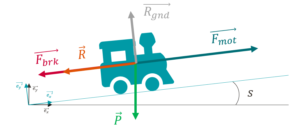
• Traction: The value of the traction force \(F_{mot}\) depends on several factors:

  • the rolling stock
  • the speed of the train, \(v^{\prime}x\) according to the effort-speed curve below:

  $$ {\vec{F_{mot}}(v_{x^{\prime}}, x^{\prime})=F_{mot}(v_{x^{\prime}}, x^{\prime})\vec{e_x^{\prime}}} $$

  

  The x axis represents the speed of the train in [km/h], the y axis the value of the traction force in [kN].

  • the action of the driver, who accelerates more or less strongly depending on where he is on his journey

• Braking : The value of the braking force \(F_{brk}\) also depends on the rolling stock and the driver’s action but has a constant value for a given rolling stock. In the current state of modelling, braking is either zero or at its maximum value.

$$ \vec{F_{brk}}(x^{\prime})=-F_{brk}(x^{\prime}){\vec{e_{x^{\prime}}}} $$

A second approach to modelling braking is the so-called hourly approach, as it is used for hourly production at SNCF. In this case, the deceleration is fixed and the braking no longer depends on the different forces applied to the train. Typical deceleration values range from 0.4 to 0.7m/s².

• Forward resistance: To model the forward resistance of the train, the Davis formula is used, which takes into account all the friction and aerodynamic resistance of the air. The value of the drag depends on the speed \(v^{\prime}_x\). The coefficients \(A\), \(B\), et \(C\) depend on the rolling stock.

$$ {\vec{R}(v_{x^{\prime}})}=-(A+Bv_{x^{\prime}}+{Cv_{x^{\prime}}}^2){\vec{e_{x^{\prime}}}} $$

• Weight (slopes + turns) : The weight force given by the product between the mass \(m\) of the train and the gravitational constant \(g\) is projected on the axes \(\vec{e_x}^{\prime}\) and \(\vec{e_y}^{\prime}\).For projection, we use the angle \(i(x^{\prime})\), which is calculated from the slope angle \(s(x^{\prime})\) corrected by a factor that takes into account the effect of the turning radius \(r(x^{\prime})\).

$$ \vec{P(x^{\prime})}=-mg\vec{e_y}(x^{\prime})= -mg\Big[sin\big(i(x^{\prime})\big){\vec{e_{x^{\prime}}}(x^{\prime})}+cos\big(i(x^{\prime})\big){\vec{e_{{\prime}}}(x^{\prime})}\Big] $$

$$ i(x^{\prime})= s(x^{\prime})+\frac{800m}{r(x^{\prime})} $$

• Ground Reaction : The ground reaction force simply compensates for the vertical component of the weight, but has no impact on the dynamics of the train as it has no component along the axis \({\vec{e_x}^{\prime}}\).

$$ \vec{R_{gnd}}=R_{gnd}{\vec{e_{y^{\prime}}}} $$

The equation of the fundamental principle of dynamics projected onto the axis \({\vec{e_x}^{\prime}}\) (in the train frame of reference) gives the following scalar equation:

$$ a_{x^{\prime}}(t) = \frac{1}{m}\Big [F_{mot}(v_{x^{\prime}}, x^{\prime})-F_{brk}(x^{\prime})-(A+Bv_{x^{\prime}}+{Cv_{x^{\prime}}}^2)-mgsin(i(x^{\prime}))\Big] $$

This is then simplified by considering that despite the gradient the train moves on a plane and by amalgamating \(\vec{e_x}\) and \(\vec{e_x}^{\prime}\). The gradient still has an impact on the force balance, but it is assumed that the train is only moving horizontally, which gives the following simplified equation:

$$ a_{x}(t) = \frac{1}{m}\Big[F_{mot}(v_{x}, x)-F_{brk}(x)-(A+Bv_{x}+{Cv_{x}}^2)-mgsin(i(x))\Big] $$

The driving force and the braking force depend on the driver’s action (he decides to accelerate or brake more or less strongly depending on the situation). This dependence is reflected in the dependence of these two forces on the position of the train. The weight component is also dependent on the position of the train, as it comes directly from the slopes and bends below the train.

In addition, the driving force depends on the speed of the train (according to the speed effort curve) as does the resistance to forward motion. resistance.

These different dependencies make it impossible to solve this equation analytically, and the acceleration of the train at each moment must be calculated by numerical integration.