Numerical integration
Introduction
Since physical modelling has shown that the acceleration of the train is influenced by various factors that vary along the route (gradient, curvature, engine traction force, etc.), the calculation must be carried out using a numerical integration method. The path is then separated into sufficiently short steps to consider all these factors as constant, which allows this time to use the equation of motion to calculate the displacement and speed of the train.
Euler’s method of numerical integration is the simplest way of doing this, but it has a number of drawbacks. This article explains the Euler method, why it is not suitable for OSRD purposes and which integration method should be used instead.
Euler’s method
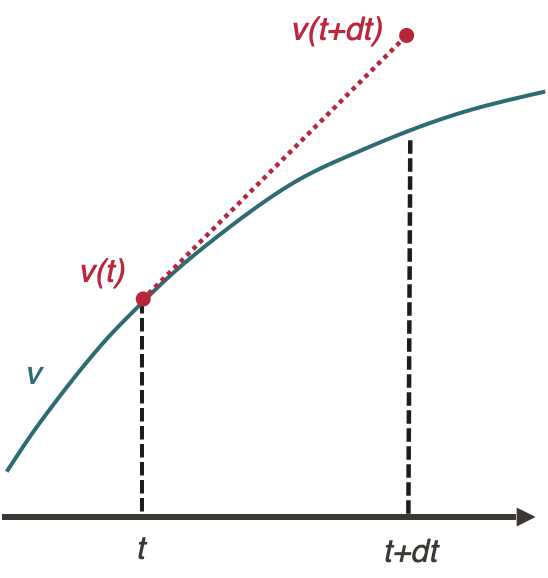
The Euler method applied to the integration of the equation of motion of a train is:
$$v(t+dt) = a(v(t), x(t))dt + v(t)$$
$$x(t+dt) = \frac{1}{2}a(v(t), x(t))dt^2 + v(t)dt + x(t)$$
Advantages of Euler’s method
The advantages of the Euler method are that it is very simple to implement and has a rather fast calculation for a given time step, compared to other numerical integration methods (see appendix)
Disadvantages of the Euler’s method
The Euler integration method presents a number of problems for OSRD:
- It is relatively imprecise, and therefore requires a small time step, which generates a lot of data.
- With time integration, only the conditions at the starting point of the integration step (gradient, infrastructure parameters, etc.) are known, as one cannot predict precisely where it will end.
- We cannot anticipate future changes in the directive: the train only reacts by comparing its current state with its set point at the same time. To illustrate, it is as if the driver is unable to see ahead, whereas in reality he anticipates according to the signals, slopes and bends he sees ahead.
Runge-Kutta’s 4 method
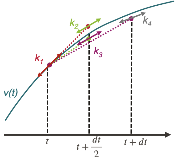
The Runge-Kutta 4 method applied to the integration of the equation of motion of a train is:
$$v(t+dt) = v(t) + \frac{1}{6}(k_1 + 2k_2 + 2k_3 + k_4)dt$$
With:
$$k_1 = a(v(t), x(t))$$
$$k_2 = a\Big(v(t+k_1\frac{dt}{2}), x(t) + v(t)\frac{dt}{2} + k_1\frac{dt^2}{8}\Big)$$
$$k_3 = a\Big(v(t+k_2\frac{dt}{2}), x(t) + v(t)\frac{dt}{2} + k_2\frac{dt^2}{8}\Big)$$
$$k_4 = a\Big(v(t+k_3dt), x(t) + v(t)dt + k_3\frac{dt^2}{2}\Big)$$
Advantages of Runge Kutta’s 4 method
Runge Kutta’s method of integration 4 addresses the various problems raised by Euler’s method:
- It allows the anticipation of directive changes within a calculation step, thus representing more accurately the reality of driving a train.
- It is more accurate for the same calculation time (see appendix), allowing for larger integration steps and therefore fewer data points.
Disadvantages of Runge Kutta’s 4 method
The only notable drawback of the Runge Kutta 4 method encountered so far is its difficulty of implementation.
The choice of integration method for OSRD
Study of accuracy and speed of calculation
Different integration methods could have replaced the basic Euler integration in the OSRD algorithm. In order to decide which method would be most suitable, a study of the accuracy and computational speed of different methods was carried out. This study compared the following methods:
- Euler
- Euler-Cauchy
- Runge-Kutta 4
- Adams 2
- Adams 3
All explanations of these methods can be found (in French) in this document, and the python code used for the simulation is here.
The simulation calculates the position and speed of a high-speed train accelerating on a flat straight line.
Equivalent time step simulations
A reference curve was simulated using the Euler method with a time step of 0.1s, then the same path was simulated using the other methods with a time step of 1s. It is then possible to simply compare each curve to the reference curve, by calculating the absolute value of the difference at each calculated point. The resulting absolute error of the train’s position over its distance travelled is as follows:
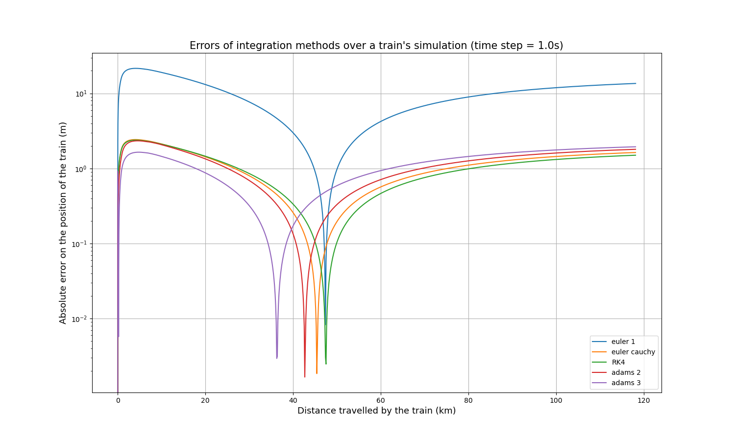
It is immediately apparent that the Euler method is less accurate than the other four by about an order of magnitude. Each curve has a peak where the accuracy is extremely high (extremely low error), which is explained by the fact that all curves start slightly above the reference curve, cross it at one point and end slightly below it, or vice versa.
As accuracy is not the only important indicator, the calculation time of each method was measured. This is what we get for the same input parameters:
| Integration method | Calculation time (s) |
|---|---|
| Euler | 1.86 |
| Euler-Cauchy | 3.80 |
| Runge-Kutta 4 | 7.01 |
| Adams 2 | 3.43 |
| Adams 3 | 5.27 |
Thus, Euler-Cauchy and Adams 2 are about twice as slow as Euler, Adams 3 is about three times as slow, and RK4 is about four times as slow. These results have been verified on much longer simulations, and the different ratios are maintained.
Simulation with equivalent calculation time
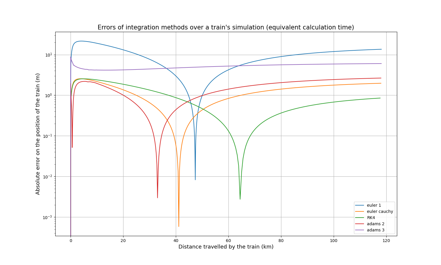
As the computation times of all methods depend linearly on the time step, it is relatively simple to compare the accuracy for approximately the same computation time. Multiplying the time step of Euler-Cauchy and Adams 2 by 2, the time step of Adams 3 by 3, and the time step of RK4 by 4, here are the resulting absolute error curves:
And here are the calculation times:
| Integration method | Calculation time (s) |
|---|---|
| Euler | 1.75 |
| Euler-Cauchy | 2.10 |
| Runge-Kutta 4 | 1.95 |
| Adams 2 | 1.91 |
| Adams 3 | 1.99 |
After some time, RK4 tends to be the most accurate method, slightly more accurate than Euler-Cauchy, and still much more accurate than the Euler method.
Conclusions of the study
The study of accuracy and computational speed presented above shows that RK4 and Euler-Cauchy would be good candidates to replace the Euler algorithm in OSRD: both are fast, accurate, and could replace the Euler method without requiring large implementation changes because they only compute within the current time step. It was decided that OSRD would use the Runge-Kutta 4 method because it is slightly more accurate than Euler-Cauchy and it is a well-known method for this type of calculation, so it is very suitable for an open-source simulator.