OSRD can be used to perform two types of calculations:
Standalone train simulation: calculation of the travel time of a train on a given route without interaction between the train and the signalling system.
Simulation: “dynamic” calculation of several trains interacting with each other via the signalling system.
1 - The input data
A running time calculation is based on 5 inputs:
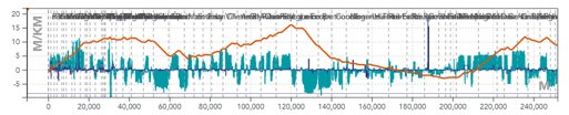
Infrastructure: Line and track topology, position of stations and passenger buildings, position and type of points, signals, maximum line speeds, corrected line profile (gradients, ramps and curves).
The blue histogram is a representation of the gradients in [‰] per position in [m]. The gradients are positive for ramps and negative for slopes.
The orange line represents the cumulative profile, i.e. the relative altitude to the starting point.
The blue line is a representation of turns in terms of radii of curves in [m].
The rolling stock: The characteristics of which needed to perform the simulation are shown below.
The orange curve, called the effort-speed curve, represents the maximum motor effort as a function of the speed of travel.
The length, mass, and maximum speed of the train are shown at the bottom of the box.
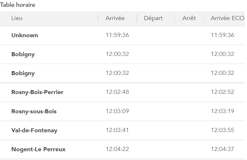
The departure time is then used to calculate the times of passage at the various points of interest (including stations).
Allowances: Time added to the train’s journey to relax its running (see page on allowances).
The results of a running time calculation can be represented in different forms:
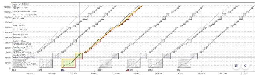
The space/time graph (GET): represents the path of trains in space and time, in the form of generally diagonal lines whose slope is the speed. Stops are shown as horizontal plates.
Example of a GET with several trains spaced about 30 minutes apart.
The x axis is the time of the train, the y axis is the position of the train in [m].
The blue line represents the most tense running calculation for the train, the green line represents a relaxed, so-called “economic” running calculation.
The solid rectangles surrounding the paths represent the portions of the track successively reserved for the train to pass (called blocks).
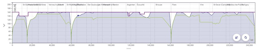
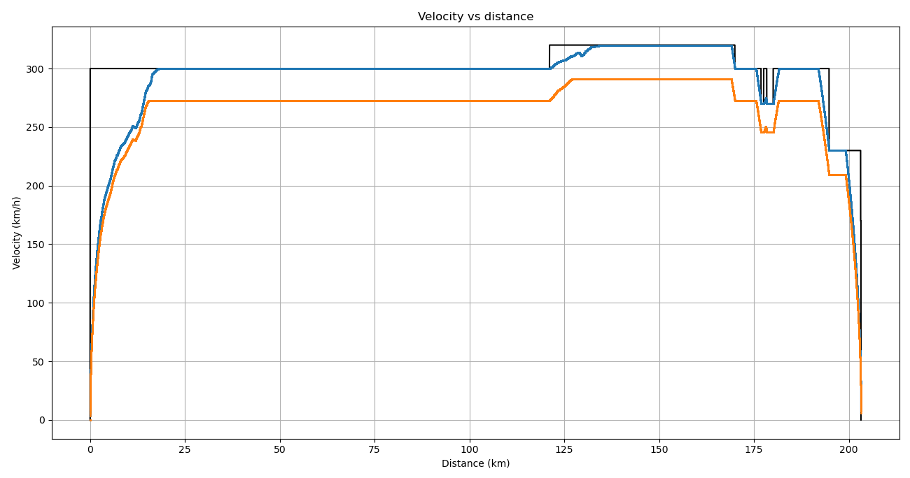
The space/speed graph (SSG): represents the journey of a single train, this time in terms of speed. Stops are therefore shown as a drop in the curve to zero, followed by a re-acceleration.
The x axis is the train position in [m], the y axis is the train speed in [km/h].
The purple line represents the maximum permitted speed.
The blue line represents the speed in the case of the most stretched running calculation.
The green line represents the speed in the case of the “economic” travel calculation.
The timetable for the passage of the train at the various points of interest.
1 - Physical modeling
Physical modelling plays an important role in the OSRD core calculation. It allows us to simulate train traffic, and it must be as realistic as possible train traffic, and it must be as realistic as possible.
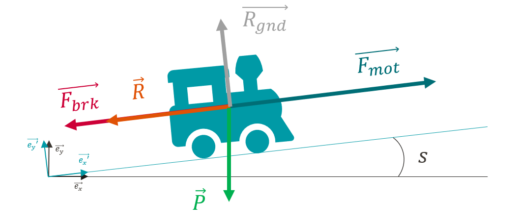
Force review
To calculate the displacement of the train over time, we must first calculate its speed at each instant.
A simple way to obtain this speed is to calculate the acceleration.
Thanks to the fundamental principle of dynamics, the acceleration of the train at each instant is directly dependent on the different forces applied to it: $$ \sum \vec{F}=m\vec{a} $$
Traction: The value of the traction force \(F_{mot}\) depends on several factors:
the rolling stock
the speed of the train, \(v^{\prime}x\) according to the effort-speed curve below:
The x axis represents the speed of the train in [km/h], the y axis the value of the traction force in [kN].
the action of the driver, who accelerates more or less strongly depending on where he is on his journey
Braking : The value of the braking force \(F_{brk}\) also depends on the rolling stock and the driver’s action but has a constant value for a given rolling stock. In the current state of modelling, braking is either zero or at its maximum value.
A second approach to modelling braking is the so-called hourly approach, as it is used for hourly production at SNCF. In this case, the deceleration is fixed and the braking no longer depends on the different forces applied to the train. Typical deceleration values range from 0.4 to 0.7m/s².
Forward resistance: To model the forward resistance of the train, the Davis formula is used, which takes into account all the friction and aerodynamic resistance of the air. The value of the drag depends on the speed \(v^{\prime}_x\). The coefficients \(A\), \(B\), et \(C\) depend on the rolling stock.
Weight (slopes + turns) : The weight force given by the product between the mass \(m\) of the train and the gravitational constant \(g\) is projected on the axes \(\vec{e_x}^{\prime}\) and \(\vec{e_y}^{\prime}\).For projection, we use the angle \(i(x^{\prime})\), which is calculated from the slope angle \(s(x^{\prime})\) corrected by a factor that takes into account the effect of the turning radius \(r(x^{\prime})\).
Ground Reaction : The ground reaction force simply compensates for the vertical component of the weight, but has no impact on the dynamics of the train as it has no component along the axis \({\vec{e_x}^{\prime}}\).
$$ \vec{R_{gnd}}=R_{gnd}{\vec{e_{y^{\prime}}}} $$
Forces balance
The equation of the fundamental principle of dynamics projected onto the axis \({\vec{e_x}^{\prime}}\) (in the train frame of reference) gives the following scalar equation:
This is then simplified by considering that despite the gradient the train moves on a plane and by amalgamating
\(\vec{e_x}\) and \(\vec{e_x}^{\prime}\). The gradient still has an impact on the force balance, but it is assumed that the train is only moving horizontally, which gives the following simplified equation:
The driving force and the braking force depend on the driver’s action (he decides to accelerate or brake more or less strongly depending on the situation). This dependence is reflected in the dependence of these two forces on the position of the train. The weight component is also dependent on the position of the train, as it comes directly from the slopes and bends below the train.
In addition, the driving force depends on the speed of the train (according to the speed effort curve) as does the resistance to forward motion.
resistance.
These different dependencies make it impossible to solve this equation analytically, and the acceleration of the train at each moment must be calculated by numerical integration.
2 - Numerical integration
Introduction
Since physical modelling has shown that the acceleration of the train is influenced by various factors that vary along the route (gradient, curvature, engine traction force, etc.), the calculation must be carried out using a numerical integration method. The path is then separated into sufficiently short steps to consider all these factors as constant, which allows this time to use the equation of motion to calculate the displacement and speed of the train.
Euler’s method of numerical integration is the simplest way of doing this, but it has a number of drawbacks. This article explains the Euler method, why it is not suitable for OSRD purposes and which integration method should be used instead.
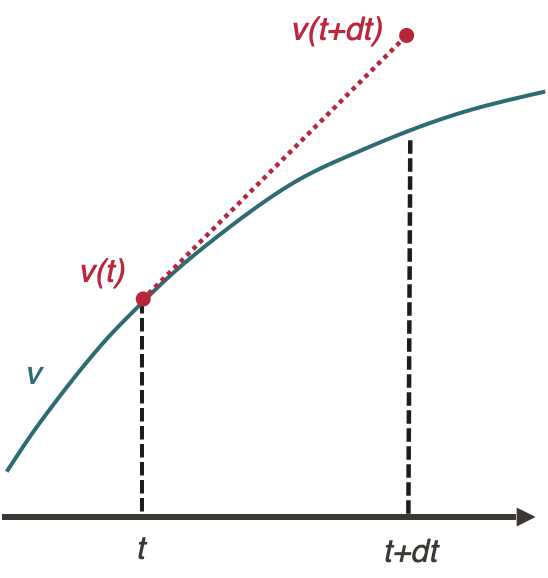
Euler’s method
The Euler method applied to the integration of the equation of motion of a train is:
The advantages of the Euler method are that it is very simple to implement and has a rather fast calculation for a given time step, compared to other numerical integration methods (see appendix)
Disadvantages of the Euler’s method
The Euler integration method presents a number of problems for OSRD:
It is relatively imprecise, and therefore requires a small time step, which generates a lot of data.
With time integration, only the conditions at the starting point of the integration step (gradient, infrastructure parameters, etc.) are known, as one cannot predict precisely where it will end.
We cannot anticipate future changes in the directive: the train only reacts by comparing its current state with its set point at the same time. To illustrate, it is as if the driver is unable to see ahead, whereas in reality he anticipates according to the signals, slopes and bends he sees ahead.
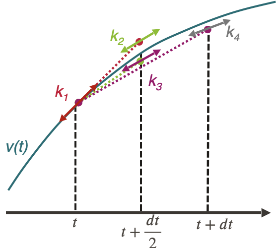
Runge-Kutta’s 4 method
The Runge-Kutta 4 method applied to the integration of the equation of motion of a train is:
Runge Kutta’s method of integration 4 addresses the various problems raised by Euler’s method:
It allows the anticipation of directive changes within a calculation step, thus representing more accurately the reality of driving a train.
It is more accurate for the same calculation time (see appendix), allowing for larger integration steps and therefore fewer data points.
Disadvantages of Runge Kutta’s 4 method
The only notable drawback of the Runge Kutta 4 method encountered so far is its difficulty of implementation.
The choice of integration method for OSRD
Study of accuracy and speed of calculation
Different integration methods could have replaced the basic Euler integration in the OSRD algorithm. In order to decide which method would be most suitable, a study of the accuracy and computational speed of different methods was carried out. This study compared the following methods:
Euler
Euler-Cauchy
Runge-Kutta 4
Adams 2
Adams 3
All explanations of these methods can be found (in French) in this document, and the python code used for the simulation is here.
The simulation calculates the position and speed of a high-speed train accelerating on a flat straight line.
Equivalent time step simulations
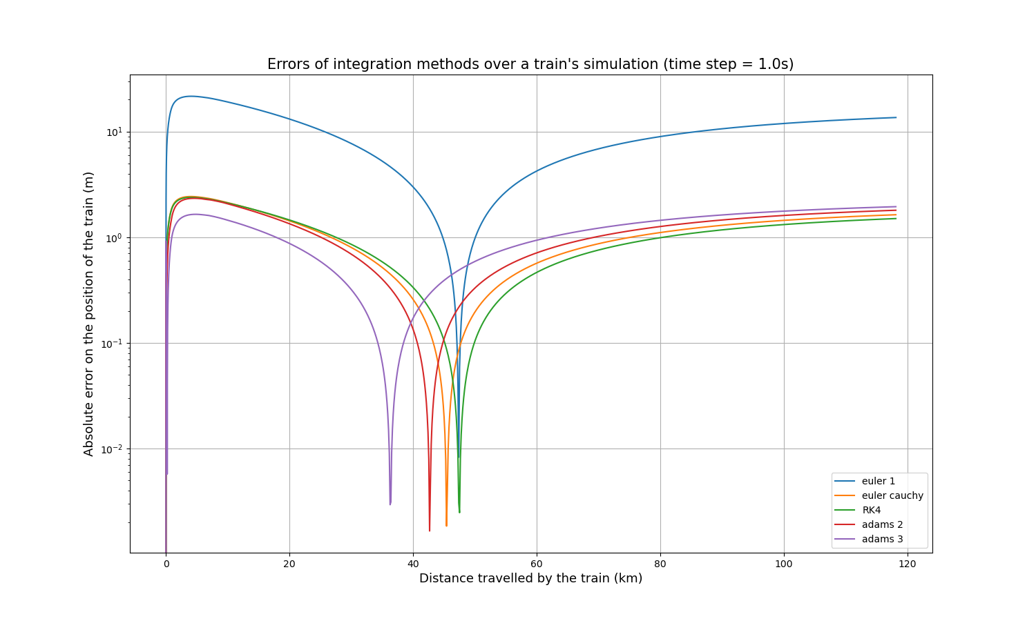
A reference curve was simulated using the Euler method with a time step of 0.1s, then the same path was simulated using the other methods with a time step of 1s. It is then possible to simply compare each curve to the reference curve, by calculating the absolute value of the difference at each calculated point. The resulting absolute error of the train’s position over its distance travelled is as follows:
It is immediately apparent that the Euler method is less accurate than the other four by about an order of magnitude. Each curve has a peak where the accuracy is extremely high (extremely low error), which is explained by the fact that all curves start slightly above the reference curve, cross it at one point and end slightly below it, or vice versa.
As accuracy is not the only important indicator, the calculation time of each method was measured. This is what we get for the same input parameters:
Integration method
Calculation time (s)
Euler
1.86
Euler-Cauchy
3.80
Runge-Kutta 4
7.01
Adams 2
3.43
Adams 3
5.27
Thus, Euler-Cauchy and Adams 2 are about twice as slow as Euler, Adams 3 is about three times as slow, and RK4 is about four times as slow. These results have been verified on much longer simulations, and the different ratios are maintained.
Simulation with equivalent calculation time
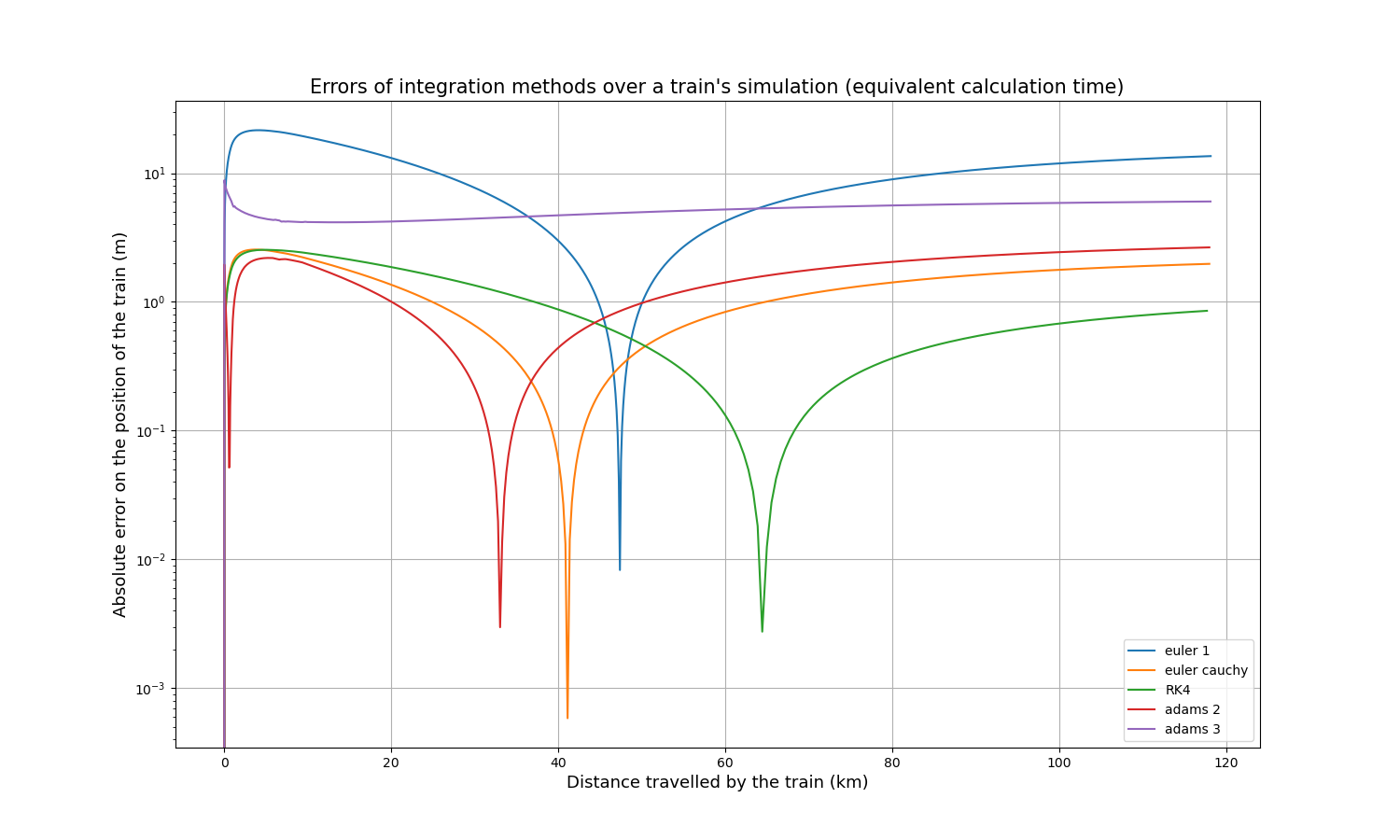
As the computation times of all methods depend linearly on the time step, it is relatively simple to compare the accuracy for approximately the same computation time. Multiplying the time step of Euler-Cauchy and Adams 2 by 2, the time step of Adams 3 by 3, and the time step of RK4 by 4, here are the resulting absolute error curves:
And here are the calculation times:
Integration method
Calculation time (s)
Euler
1.75
Euler-Cauchy
2.10
Runge-Kutta 4
1.95
Adams 2
1.91
Adams 3
1.99
After some time, RK4 tends to be the most accurate method, slightly more accurate than Euler-Cauchy, and still much more accurate than the Euler method.
Conclusions of the study
The study of accuracy and computational speed presented above shows that RK4 and Euler-Cauchy would be good candidates to replace the Euler algorithm in OSRD: both are fast, accurate, and could replace the Euler method without requiring large implementation changes because they only compute within the current time step.
It was decided that OSRD would use the Runge-Kutta 4 method because it is slightly more accurate than Euler-Cauchy and it is a well-known method for this type of calculation, so it is very suitable for an open-source simulator.
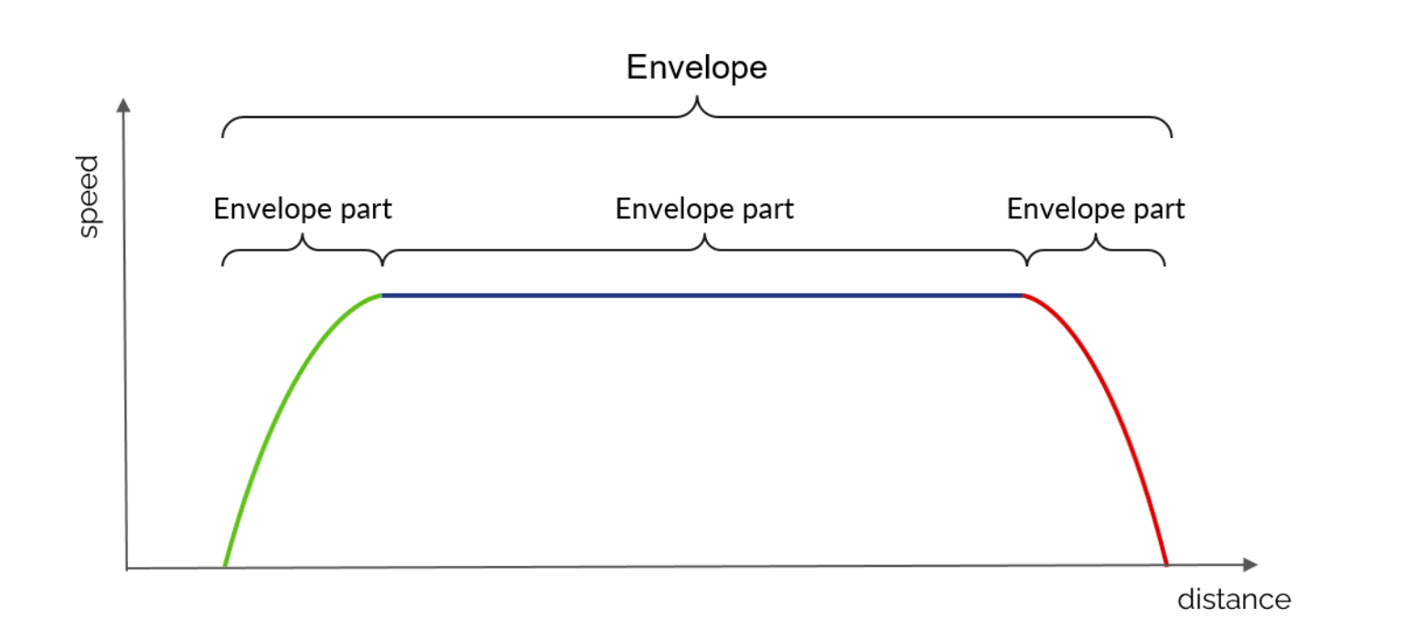
3 - Envelopes system
The envelope system is an interface created specifically for the OSRD gait calculation. It allows you to manipulate different space/velocity curves, to slice them, to end them, to interpolate specific points, and to address many other needs necessary for the gait calculation.
A specific interface in the OSRD Core service
The envelope system is part of the core service of OSRD (see software architecture).
Its main components are :
1 - EnvelopePart: space/speed curve, defined as a sequence of points and having metadata indicating for example if it is an acceleration curve, a braking curve, a speed hold curve, etc.
2 - Envelope: a list of end-to-end EnvelopeParts on which it is possible to perform certain operations:
check for continuity in space (mandatory) and speed (optional)
look for the minimum and/or maximum speed of the envelope
cut a part of the envelope between two points in space
perform a velocity interpolation at a certain position
calculate the elapsed time between two positions in the envelope
3 - Overlays : system for adding more constrained (i.e. lower speed) EnvelopeParts to an existing envelope.
Given envelopes vs. calculated envelopes
During the simulation, the train is supposed to follow certain speed instructions. These are modelled in OSRD by envelopes in the form of space/speed curves. Two types can be distinguished:
Envelopes from infrastructure and rolling stock data, such as maximum line speed and maximum train speed. Being input data for our calculation, they do not correspond to curves with a physical meaning, as they are not derived from the results of a real integration of the physical equations of motion.
The envelopes result from real integration of the physical equations of motion. They correspond to a curve that is physically tenable by the train and also contain time information.
A simple example to illustrate this difference: if we simulate a TER journey on a mountain line, one of the input data will be a maximum speed envelope of 160km/h, corresponding to the maximum speed of our TER. However, this envelope does not correspond to a physical reality, as it is possible that on certain sections the gradient is too steep for the train to be able to maintain this maximum speed of 160km/h. The calculated envelope will therefore show in this example a speed drop in the steepest areas, where the envelope given was perfectly flat.
Simulation of several trains
In the case of the simulation of many trains, the signalling system must ensure safety. The effect of signalling on the running calculation of a train is reproduced by superimposing dynamic envelopes on the static envelope. A new dynamic envelope is introduced for example when a signal closes. The train follows the static economic envelope superimposed on the dynamic envelopes, if any. In this simulation mode, a time check is performed against a theoretical time from the time information of the static economic envelope. If the train is late with respect to the scheduled time, it stops following the economic envelope and tries to go faster. Its space/speed curve will therefore be limited by the maximum effort envelope.
4 - Pipeline
The walk calculation in OSRD is a 4-step process, each using the envelopes system:
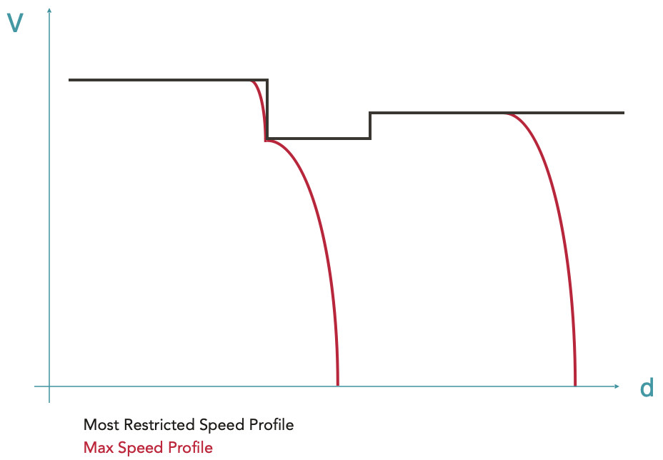
Calculation of the Most Restricted Speed Profile (MRSP)
A first envelope is calculated at the beginning of the simulation by grouping all static velocity limits:
maximum line speed
maximum speed of rolling stock
temporary speed limits (e.g. in case of works on a line)
speed limits by train category
speed limits according to train load
speed limits corresponding to signposts
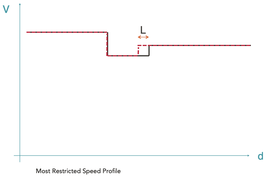
The length of the train is also taken into account to ensure that the train does not accelerate until its tail leaves the slowest speed zone. An offset is then applied to the red dashed curve. The resulting envelope (black curve) is called the Most Restricted Speed Profile (MRSP). It is on this envelope that the following steps will be calculated.
The red dotted line represents the maximum permitted speed depending on the position.
The black line represents the MRSP where the train length has been taken into account.
It should be noted that the different envelopeParts composing the MRSP are input data, so they do not correspond to curves with a physical reality.
Calculation of the Max Speed Profile
Starting from the MRSP, all braking curves are calculated using the overlay system (see here for more details on overlays), i.e. by creating envelopeParts which will be more restrictive than the MRSP. The resulting curve is called Max Speed Profile. This is the maximum speed envelope of the train, taking into account its braking capabilities.
Since braking curves have an imposed end point and the braking equation has no analytical solution, it is impossible to predict their starting point. The braking curves are therefore calculated backwards from their target point, i.e. the point in space where a certain speed limit is imposed (finite target speed) or the stopping point (zero target speed).
For historical reasons in hourly production, braking curves are calculated at SNCF with a fixed deceleration, the so-called hourly deceleration (typically ~0.5m/s²) without taking into account the other forces. This method has therefore also been implemented in OSRD, allowing the calculation of braking in two different ways: with this hourly rate or with a braking force that is simply added to the other forces.
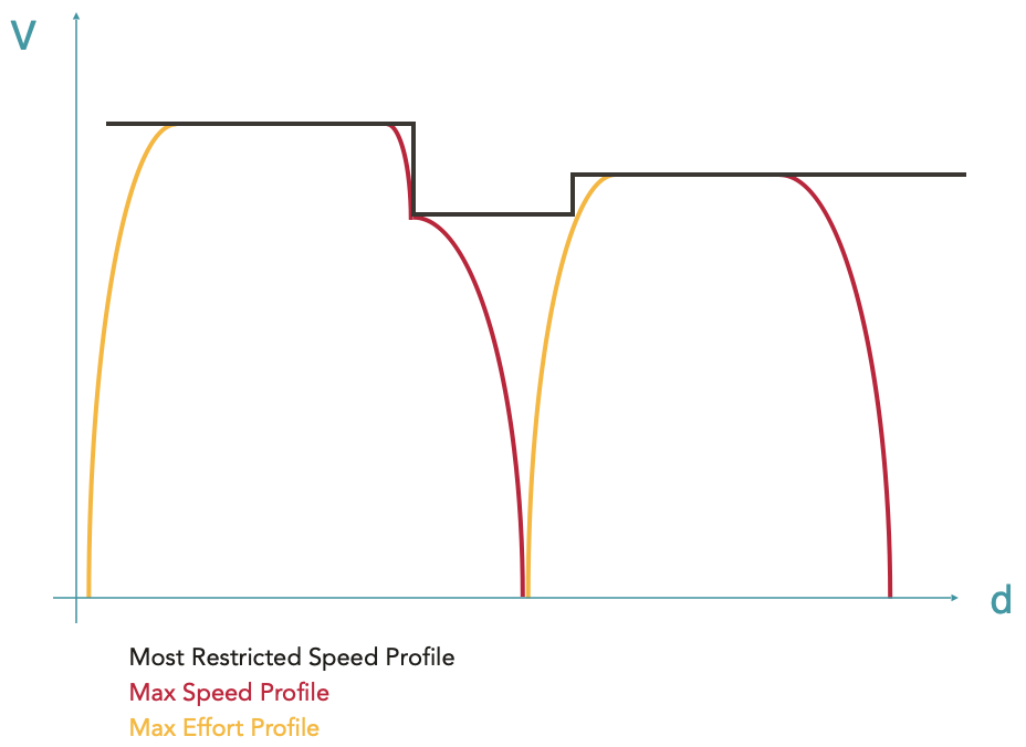
Calculation of the Max Effort Profile
For each point corresponding to an increase in speed in the MRSP or at the end of a stop braking curve, an acceleration curve is calculated. The acceleration curves are calculated taking into account all active forces (traction force, driving resistance, weight) and therefore have a physical meaning.
For envelopeParts whose physical meaning has not yet been verified (which at this stage are the constant speed running phases, always coming from the MRSP), a new integration of the equations of motion is performed. This last calculation is necessary to take into account possible speed stalls in case the train is physically unable to hold its speed, typically in the presence of steep ramps (see this example).
The envelope that results from the addition of the acceleration curves and the verification of the speed plates is called the Max Effort Profile.
At this stage, the resulting envelope is continuous and has a physical meaning from start to finish. The train accelerates to the maximum, runs as fast as possible according to the different speed limits and driving capabilities, and brakes to the maximum. The resulting travel calculation is called the basic running time. It corresponds to the fastest possible route for the given rolling stock on the given route.
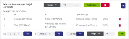
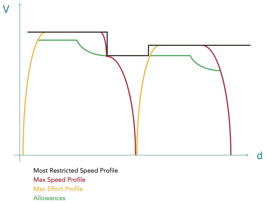
Application of allowance(s)
After the calculation of the basic run (corresponding to the Max Effort Profile in OSRD), it is possible to apply allowances. Allowances are additions of extra time to the train’s journey. They are used to allow the train to catch up if necessary or for other operational purposes (more details on allowances here).
A new Allowances envelope is therefore calculated using overlays to distribute the allowance requested by the user over the maximum effort envelope calculated previously.
In the OSRD running calculation it is possible to distribute the allowances in a linear way, by lowering all speeds by a certain factor, or in an economic way, i.e. by minimising the energy consumption during the train run.
5 - Allowances
The purpose of allowances
As explained in the calculation of the Max Effort Profile, the basic running time represents the most stretched run normally achievable, i.e. the fastest possible run of the given equipment on the given route. The train accelerates to the maximum, travels as fast as possible according to the different speed limits and driving capabilities, and brakes to the maximum.
This basic run has a major disadvantage: if a train leaves 10 minutes late, it will arrive at best 10 minutes late, because by definition it is impossible for it to run faster than the basic run. Therefore, trains are scheduled with one or more allowances added. The allowances are a relaxation of the train’s route, an addition of time to the scheduled timetable, which inevitably results in a lowering of running speeds.
A train running in basic gear is unable to catch up!
Allowances types
There are two types of allowances:
The regularity allowance: this is the additional time added to the basic running time to take account of the inaccuracy of speed measurement, to compensate for the consequences of external incidents that disrupt the theoretical run of trains, and to maintain the regularity of the traffic. The regularity allowance applies to the whole route, although its value may change at certain intervals.
The construction allowance: this is the time added/removed on a specific interval, in addition to the regularity allowance, but this time for operational reasons (dodging another train, clearing a track more quickly, etc.)
A basic running time with an added allowance of regularity gives what is known as a standard walk.
Allowance distribution
Since the addition of allowance results in lower speeds along the route, there are a number of possible routes. Indeed, there are an infinite number of solutions that result in the same journey time.
As a simple example, in order to reduce the running time of a train by 10% of its journey time, it is possible to extend any stop by the time equivalent to this 10%, just as it is possible to run at 1/1.1 = 90.9% of the train’s capacity over the entire route, or to run slower, but only at high speeds…
There are currently two algorithms for margin distribution in OSRD: linear and economic.
Linear distribution
Linear allowance distribution is simply lowering the speeds by the same factor over the area where the user applies the allowance. Here is an example of its application:
The advantage of this distribution is that the allowance is spread evenly over the entire journey. A train that is late on 30% of its journey will have 70% of its allowance for the remaining 70% of its journey.
Economic distribution
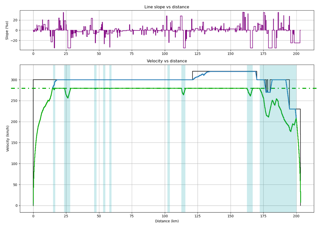
The economic distribution of the allowance, presented in detail in this document (MARECO is an algorithm designed by the SNCF research department), consists of distributing the allowance in the most energy-efficient way possible. It is based on two principles:
a maximum speed, avoiding the most energy-intensive speeds
run-on zones, located before braking and steep gradients, where the train runs with the engine off thanks to its inertia, allowing it to consume no energy during this period
An example of economic walking. Above, the gradients/ramps encountered by the train. The areas of travel on the track are shown in blue.