Explanations discuss key topics and concepts at a fairly high level and provide useful background information and explanation.
This is the multi-page printable view of this section. Click here to print.
Explanations
Learn more about key concepts
- 1: Containers architecture
- 2: Models
- 3: Running time calculation
- 3.1: Physical modeling
- 3.2: Numerical integration
- 3.3: Envelopes system
- 3.4: Pipeline
- 3.5: Allowances
- 4: Netzgrafik-Editor
1 - Containers architecture
How the containers works together and how they are built
There are 3 main containers deployed in a standard OSRD setup:
- Gateway (includes the frontend): Serves the front end, handles authentication and proxies requests to the backend.
- Editoast: Acts as the backend that interacts with the front end.
- Core: Handles computation and business logic, called by Editoast.
Standard deployment
The standard deployment can be represented with the following diagram.
flowchart TD
    gw["gateway"]
    front["front-end static files"]
    gw -- local file --> front

    browser --> gw
    gw -- HTTP --> editoast
    editoast -- HTTP --> core
External requests are received by the gateway. If the path asked starts with /api it will be forwarded using HTTP to editoast, otherwise it will serve a file with the asked path. Editoast reach the core using HTTP if required.
The gateway is not only a reverse proxy with the front-end bundle included, it also provides all the authentication mechanisms: using OIDC or tokens.
2 - Models
What is modeled in OSRD, and how it is modeled
2.1 - Infrastructure example
Explains using an example how infrastructure data is structured
Introduction
This page gives an example of how the data formats are used to describe an infrastructure in OSRD.
For this purpose, let’s take as an example the following toy infrastructure:

Tip
To zoom in on diagrams, click on the edit button that appears when hovering over it.This diagram is an overview of the infrastructure with lines and stations only.
This infrastructure is not meant to be realistic, but rather meant to help illustrate OSRD’s data model. This example will be created step by step and explained along the way.
The infrastructure generator
In the OSRD repository is a python library designed to help generate infrastructures in a format understood by OSRD.
The infrastructure discussed in this section can be generated thanks to small_infra.py file. To learn more about the generation scripts, you can check out the related README.
Tracks
Track sections
The first objects we need to define are TrackSections. Most other objects are positioned relative to track sections.
A track section is a section of rail (switches not included). One can chose to divide the tracks of their infrastructure in as many track sections as they like. Here we chose to use the longest track sections possible, which means that between two switches there is always a single track section.
Track sections is what simulated trains roll onto. They are the abstract equivalent to physical rail sections. Track sections are bidirectional.
In this example, we define two tracks for the line between the West and North-East stations. We also have overpassing tracks at the North and Mid-West stations for added realism. Finally, we have three separate tracks in the West station, since it’s a major hub in our imaginary infrastructure.

Important
TrackSections are represented as arrows in this diagram to stress the fact that they have a start and an end. It matters as objects positioned on track sections are located using their distance from the start of their track section.
Therefore, to locate an object at the beginning of its track section, set its offset to 0. To move it to the end of its track section, set its offset to the length of the track section.
These attributes are required for the track section to be complete:
length: the length of the track section in meters.geo: the coordinates in real life (geo is for geographic), in the GeoJSON format.- cosmetic attributes:
line_name,track_name,track_numberwhich are used to indicate the name and labels that were given to the tracks / lines in real life.
For all track sections in our infrastructure, the geo attributes very much resemble the given diagram.
For most track sections, their length is proportional to what can be seen in the diagram. To preserve readability, exceptions were made for TA6, TA7, TD0 and TD1 (which are 10km and 25km).
Node
A Node represents a node in the infrastructure. In an OSRD simulation, a train can only move from one section of track to another if they are linked by a node.
Node Types
NodeTypes have two mandatory attributes:
ports: A list of port names. A port is an endpoint connected to a track section.groups: A mapping between group names and lists of branch (connection between 2 ports) that characterises the different possible positions of the node type
At any time, all nodes have an active group, and may have an active branch, which always belongs to the active group. During a simulation, changing the active branch inside a group is instantaneous, but changing the active branch across groups (changing the active group) takes configurable time.
This is because a node is a physical object, and changing active branch can involve moving parts of it. Groups are designed to represent the different positions that a node can have. Each group contains the branches that can be used in the associated node position.
The duration needed to change group is stored inside the Node, since it can vary depending on the physical implementation of the node.
Our examples currently use five node types. Node types are just like other objects, and can easily be added as needed using extended_switch_type.
1) Link
This one represents the link between two sections of track. It has two ports: A and B.

It is used in the OSRD model to create a link between two track sections. This is not a physical object.
2) The Point Switch
The ubiquitous Y switch, which can be thought of as either two tracks merging, or one track splitting.
This node type has three ports: A, B1 and B2.

There are two groups, each with one connection in their list: A_B1, which connects A to B1, and A_B2 which connects A to B2.
Thus, at any given moment (except when the switch moves from one group to another), a train can go from A to B1 or from A to B2 but never to both at the same time. A train cannot go from B1 to B2.
A Point Switch only has two positions:
- A to B1
- A to B2


3) The Crossing
This is simply two tracks crossing each other.
This type has four ports: A1, B1, A2 et B2.

It has only one group containing two connections: A1 to B1 and A2 to B2. Indeed this kind of switch is passive: it has no moving parts. Despite having a single group, it is still used by the simulation to enforce route reservations.
Here are the two different connections this switch type has:
- A1 to B1
- A2 to B2


4) The Double slip switch
This one is more like two point switches back to back. It has four ports: A1, A2, B1 and B2.

However, it has four groups, each with one connection. The four groups are represented in the following diagram:
- A1 to B1
- A1 to B2
- A2 to B1
- A2 to B2


5) The Single slip switch
This one looks more like a cross between a single needle and a crossover. It has four ports: A1, A2, B1 and B2.

Here are the three connections that can be made by this switch:
- A1 to B1
- A1 to B2
- A2 to B2


Back to nodes
A Node has three attributes:
node_type: the identifier of theNodeTypeof this node.ports: a mapping from port names to track sections extremities.group_change_delay: the time it takes to change which group of the node is activated.
The port names must match the ports of the node type chosen. The track section endpoints can be start or end, be careful to chose the appropriate ones.
Most of our example’s nodes are regular point switches. The path from North station to South station has two cross switches. Finally, there is a double cross switch right before the main line splits into the North-East and South-East lines.

It is important to note that these node types are hard-coded into the project code. Only the extended_node_type added by the user will appear in the railjson.
Curves and slopes
Curves and Slopes are instrumental to realistic simulations. These objects are defined as a range between a begin and end offsets of one track section. If a curve / slope spans more than one track section, it has to be added to all of them.
The slope / curve values are constant on their entire range. For varying curves / slopes, one needs to create several objects.
Slope values are measured in meters per kilometers, and the curve values are measured in meters (the radius of the curve).
Mind that the
begin value should always be smaller than the end value. That is why the curve / slope values can be negative: an uphill slope of 1 going from offset 10 to 0 is the same as a downhill slope of -1 going from offsets 0 to 10.In the small_infra.py file, we have slopes on the track sections TA6, TA7, TD0 and TD1.
There are curves as well, on the track sections TE0, TE1, TE3 and TF1.
Interlocking
All objects so far contributed to track topology (shape). Topology would be enough for trains to navigate the network, but not enough to do so safely. To ensure safety, two systems collaborate:
- Interlocking ensures trains are allowed to move forward
- Signaling is the mean by which interlocking communicates with the train
Detectors
These objects are used to create TVD sections (Track Vacancy Detection section): the track area in between detectors is a TVD section. When a train runs into a detector, the section it is entering becomes occupied. The only function of TVD sections is to locate trains.
In real life, detectors can be axle counters or track circuits for example.
For this mean of location to be efficient, detectors need to be placed regularly along your tracks, not too many because of cost, but not too few, because then TVD sections would be very large and trains would need to be very far apart to be told apart, which reduces capacity.
There often are detectors close to all sides of switches. This way, interlocking is made aware pretty much immediately when a switch is cleared, which is then free to be used again.
Let’s take a cross switch as an example: if train A is crossing it north to south and train B is coming to cross west to east, then as soon as train A’s last car has passed the crossing, B should be able to go, since A is now on a completely unrelated track section.
In OSRD, detectors are point objects, so all the attributes it needs are its id, and track location (track and offset).

The clumped up squares represent many detectors at once. Indeed, because some track sections are not represented with their full length, we could not represent all the detectors on the corresponding track section.
Some notes:
- Between some points, we added only one detector (and not two), because they were really close together, and it would have made no sense to create a tiny TVDS between the two. This situation happened on track sections (TA3, TA4, TA5, TF0 and TG3).
- In our infrastructure, there are relatively few track sections which are long enough to require more detectors than just those related to switches. Namely, TA6, TA7, TDO, TD1, TF1, TG1 and TH1. For example TD0, which measures 25km, has in fact 17 detectors in total.
Buffer stops
BufferStops are obstacles designed to prevent trains from sliding off dead ends.
In our infrastructure, there is a buffer stop on each track section which has a loose end. There are therefore 8 buffer stops in total.
Together with detectors, they set the boundaries of TVD sections (see Detectors)
Routes
A Route is an itinerary in the infrastructure. A train path is a sequence of routes. Routes are used to reserve section of path with the interlocking. See the dedicated documentation.
It is represented with the following attributes:
entry_pointandexit_point: references detectors or buffer stops which mark the beginning and the end of the Route.entry_point_direction: Direction on a track section to start the route from theentry_point.switches_direction: A set of directions to follow when we encounter a switch on our Route, to build this Route fromentry_pointtoexit_point.release_detectors: When a train clears a release detector, resources reserved from the beginning of the route until this detector are released.
Signaling
Thanks to interlocking, trains are located and allowed to move. It’s a good start, but meaningless until trains are made aware of it. This is where Signals come into play: signals react to interlocking, and can be seen by trains.
How trains react to signals depends on the aspect, kind of signal, and signaling system.
Here are the most important attributes for signals:
linked_detector: The linked detector.type_code: The type of signal.direction: The direction it protects, which can simply be interpreted as the way in which it can be seen by an incoming train (since there are lights only on one side…). Direction is relative to track section orientation.- Cosmetic attributes like
angle_geoorsidewhich control the way in which the signals are displayed in the front-end.
Here is a visualization of how one can represent a signal, and which direction it protects.

The way the signals are arranged is highly dependent on both signaling system and infrastructure manager.
Here are the basic rules used for this example infrastructure:
- We add two spacing signals (one per direction) for each detector that is cutting a long TVD section into smaller ones.
- Switch entries where a train might have to stop are protected by a signal (which is located outside of the switch TVD section). It must be visible from the direction used to approach the switch. When there are multiple switches in a row, only the first one usually needs protection, as interlocking is usually designed as not to encourage trains stopping in the middle of intersections.
Note that detectors linked to at least one signal are not represented, as there are not signals without associated detectors in this example.
To get the id of a detector linked to a signal, take the signal’s id and replace S by D (e.g. SA0 -> DA0).

On TA6, TA7, TD0 and TD1 we could not represent all signals because these track sections are very long and have many detectors, hence many signals.
Electrification
To allow electric trains to run on our infrastructure, we need to specify which parts of the infrastructure is electrified.
Catenaries
Catenaries are objects that represent the overhead wires that power electric trains. They are represented with the following attributes:
voltage: A string representing the type of power supply used for electrificationtrack_ranges: A list of range of track sections (TrackRanges) covered by this catenary. ATrackRangeis composed of a track section id, abeginoffset and anendoffset.
In our example infrastructure, we have two Catenaries:
- One with
voltageset to"1500", which covers only TA0. - One with
voltageset to"25000", which covers all others except TD1.
This means that only thermal trains can cross the TD1 track section.
Our example also outlines that, unlike its real life counterpart, a single Catenary may cover the whole infrastructure.
Neutral Sections
In some parts of an infrastructure, the train drivers may be instructed - mainly for safety reasons - to cut the power supply to the train.
To represent such parts, we use NeutralSections. They are represented mainly with the following attributes:
track_ranges: A list ofDirectedTrackRanges(track ranges associated to a direction) which are covered by this neutral section.lower_pantograph: A boolean indicating whether the train’s pantograph should be lowered while in this section.
In our example infrastructure, we have three NeutralSections: one at the junction of the "1500" and "25000" catenaries, one on TA6 and one on TG1 and TG4.
For more details about the model see the dedicated page.
Miscellaneous
Operational points
Operational point is also known in French as “Point Remarquable” (PR).
One OperationalPoint is a collection of points (OperationalPointParts) of interest.
For example, it may be convenient (reference point for train operation) to store the location of platforms as parts and group them by station in operational points.
In the same way, a bridge over tracks will be one OperationalPoint, but it will have several OperationPointParts, one at the intersection of each track. The local_track_name field provides a human-friendly track label in the context of the operational point.
In the example infrastructure, we only used operational points to represent stations. Operational point parts are displayed as purple diamonds. Keep in mind a single operational point may contain multiple parts.

Loading Gauge Limits
These objects are akin to Slopes and Curves: it covers a range of track section, with a begin and an end offset. It represents a restriction on the trains that can travel on the given range, by weight or by train type (freight or passenger).
We did not put any in our examples.
Speed Sections
The SpeedSections represent speed limits (in meters per second) that are applied on some parts of the tracks. One SpeedSection can span on several track sections, and do not necessarily cover the whole track sections. Speed sections can overlap.
In our example infrastructure, we have a speed section covering the whole infrastructure, limiting the speed to 300 km/h. On a smaller part of the infrastructure, we applied more restrictive speed sections.

2.2 - Neutral Sections
Documentation about what they are and how they are implemented
Physical object to model
Introduction
For a train to be able to run, it must either have an energy source on board (fuel, battery, hydrogen, …) or be supplied with energy throughout its journey.
To supply this energy, electrical cables are suspended above the tracks: the catenaries. The train then makes contact with these cables thanks to a conducting piece mounted on a mechanical arm: the pantograph.
Neutral sections
With this system it is difficult to ensure the electrical supply of a train continuously over the entire length of a line. On certain sections of track, it is necessary to cut the electrical supply of the train. These portions are called neutral sections.
Indeed, in order to avoid energy losses along the catenaries, the current is supplied by several substations distributed along the tracks. Two portions of catenaries supplied by different substations must be electrically isolated to avoid short circuits.
Moreover, the way the tracks are electrified (DC or not for example) can change according to the local uses and the time of installation. It is again necessary to electrically isolate the portions of tracks which are electrified differently. The train must also (except in particular cases) change its pantograph when the type of electrification changes.
In both cases, the driver is instructed to cut the train’s traction, and sometimes even to lower the pantograph.
In the French infrastructure, these zones are indicated by announcement, execution and end signs. They also carry the indication to lower the pantograph or not. The portions of track between the execution and end may not be electrified entirely, and may not even have a catenary (in this case the zone necessarily requires lowering the pantograph).
REV (for reversible) signs are sometimes placed downstream of the end of zone signs. They are intended for trains that run with a pantograph at the rear of the train. These signs indicate that the driver can resume traction safely.
Additionally, it may sometimes be impossible on a short section of track to place a catenary or to raise the train’s pantograph. In this case the line is still considered electrified, and the area without electrification (passage under a bridge for example) is considered as a neutral section.
Rolling stock
After passing through a neutral section, a train must resume traction. This is not immediate (a few seconds), and the necessary duration depends on the rolling stock.
In addition, the driver must, if necessary, lower his pantograph, which also takes time (a few tens of seconds) and also depends on the rolling stock.
Thus, the coasting imposed on the train extends outside the neutral section, since these system times are to be counted from the end of the neutral section.
Data model
We have chosen to model the neutral sections as the space between the signs linked to it (and not as the precise zone where there is no catenary or where the catenary is not electrified).
This zone is directional, i.e. associated with a direction of travel, in order to be able to take into account different placements of signs according to the direction. The execution sign of a given direction is not necessarily placed at the same position as the end of zone sign of the opposite direction.
For a two-way track, a neutral section is therefore represented by two objects.
The schema is the following
{
    "lower_pantograph": boolean,
    "track_ranges": [
        {
            "track": string,
            "start": number,
            "end": number,
            "direction": enum
        }
    ],
    "announcement_track_ranges": [
        {
            "track": string,
            "start": number,
            "end": number,
            "direction": enum
        }
    ]
}
lower_pantograph: indicates whether the pantograph should be lowered in this sectiontrack_ranges: list of track sections ranges where the train must not tractionannouncement_track_ranges: list of track sections ranges between the announcement sign and the execution sign
Display
Map
The zones displayed in the map correspond to the track_ranges of neutral sections, thus are between the execution and end signs of the zone. The color of the zone indicates whether the train must lower its pantograph in the zone or not.
The direction in which the zone applies is not represented.
Simulation results
In the linear display, it is always the area between EXE and FIN that is displayed.
Pathfinding
Neutral sections are therefore portions of “non-electrified” track where an electric train can still run (but where it cannot traction).
When searching for a path in the infrastructure, an electric train can travel through a track section that is not covered by the track_ranges of a catenary object (documentation to be written) only if it is covered by the track_ranges of a neutral section.
Simulation
In our simulation, we approximate the driver’s behavior as follows:
- The coasting is started as soon as the train’s head passes the announcement sign
- The system times (pantograph reading and traction resumption) start as soon as the train’s head passes the end sign.
In the current simulation, it is easier to use spatial integration bounds rather than temporal ones. We make the following approximation: when leaving the neutral section, we multiply the system times by the speed at the exit of the zone. The coasting is then extended over the obtained distance. This approximation is reasonable because the train’s inertia and the almost absence of friction guarantee that the speed varies little over this time interval.
Improvements to be made
Several aspects could be improved:
- We do not model the REV signs, all trains therefore only have one pantograph at the front in our simulations.
- System times are approximated.
- The driver’s behavior is rather restrictive (coasting could start after the announcement sign).
- The display of the zones is limited: no representation of the direction or the announcement zones.
- These zones are not editable.
2.3 - Rolling stock categories
Defines rolling stock categories
Categories are groupings of rolling stock, either by their characteristics, performance or by the nature of the services for which they have been designed or are used.
The same rolling stock can be used for different types of operations and services. This versatility is reflected in the following attributes:
primary_category(required) indicates the main use of a rolling stockother_categories(optional) indicates other possible uses of a rolling stock
The primary category of a rolling stock enables several features, such as filtering, differentiated display on charts or network graphic views, and, more broadly, the aggregation of rolling stocks.
Categories of rolling stocks
The different default rolling stock categories are as follows:
High-speed train(see High-speed train)Intercity train(see Intercity train)Regional train(see Regional train)Commuter train(see Commuter train)Freight train(see Freight train)Fast freight train(same as Freight train, but with a different composition code,ME140instead ofMA100for example)Night train(see Night train)Tram-train(see Tram-train)Touristic train(see Touristic train)Work train(see Work train)
It is also planned that, in the future, a user will be able to create new rolling stock categories directly.
Realistic open data rolling stocks
To make the application more accessible to users outside the railway industry, such as external contributors and research laboratories, and to prepare for the release of the public playground version of OSRD, several rolling stock created with mock data are available to all users.
These rolling stocks are designed to cover most simulation scenarios that users may encounter.
These rolling stocks are not actual rolling stocks, due to confidentiality reasons, but they have been created based on real data to ensure a high level of realism.
The rolling stocks are provided as JSON files. We created one representative rolling stock for each category listed above.
The characteristics of these rolling stocks have been calculated based on the average values of real rolling stocks within each category. Additionally, most of these models are designed to be compatible across various networks: they are primarily bi-mode (supporting multiple electric voltage and current supply types), which is not always the case for real-world rolling stocks.
An example of rolling stock, a high-speed train, is represented below, from the rolling stock editor of the application:
Open data
Since these rolling stocks are fictional (yet realistic), they can be freely used in projects beyond OSRD.
To access and use them in the application:
From the open-source playground: The rolling stocks are available by default.
From a locally launched application: Use the corresponding command in the README to import the test rolling stocks in your database.
3 - Running time calculation
OSRD can be used to perform two types of calculations:
- Standalone train simulation: calculation of the travel time of a train on a given route without interaction between the train and the signalling system.
- Simulation: “dynamic” calculation of several trains interacting with each other via the signalling system.
1 - The input data
A running time calculation is based on 5 inputs:
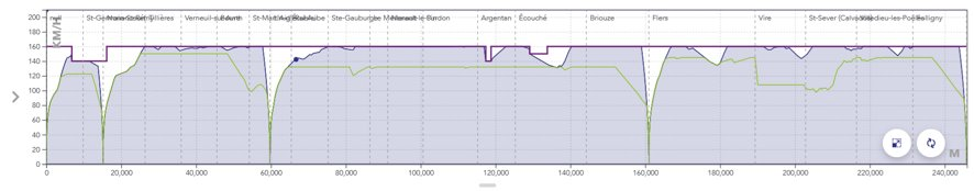
- Infrastructure: Line and track topology, position of stations and passenger buildings, position and type of points, signals, maximum line speeds, corrected line profile (gradients, ramps and curves).
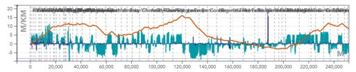
The blue histogram is a representation of the gradients in [‰] per position in [m]. The gradients are positive for ramps and negative for slopes.
The orange line represents the cumulative profile, i.e. the relative altitude to the starting point.
The blue line is a representation of turns in terms of radii of curves in [m].
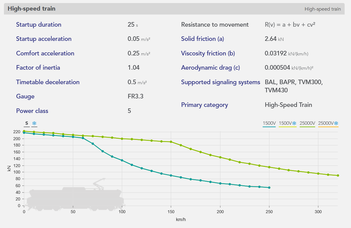
- The rolling stock: The characteristics of which needed to perform the simulation are shown below.

The orange curve, called the effort-speed curve, represents the maximum motor effort as a function of the speed of travel.
The length, mass, and maximum speed of the train are shown at the bottom of the box.
The departure time is then used to calculate the times of passage at the various points of interest (including stations).
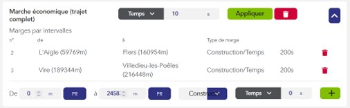
Allowances: Time added to the train’s journey to relax its running (see page on allowances).
- The time step for the calculation of numerical integration.
2 - The results
The results of a running time calculation can be represented in different forms:
- The space/time graph (GET): represents the path of trains in space and time, in the form of generally diagonal lines whose slope is the speed. Stops are shown as horizontal plates.
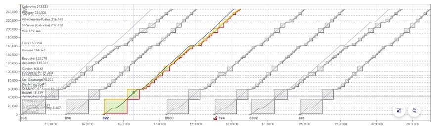
Example of a GET with several trains spaced about 30 minutes apart.
The x axis is the time of the train, the y axis is the position of the train in [m].
The blue line represents the most tense running calculation for the train, the green line represents a relaxed, so-called “economic” running calculation.
The solid rectangles surrounding the paths represent the portions of the track successively reserved for the train to pass (called blocks).
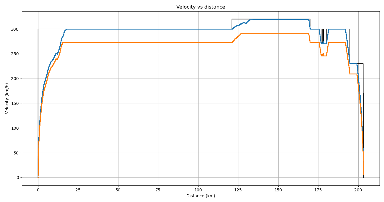
- The space/speed graph (SSG): represents the journey of a single train, this time in terms of speed. Stops are therefore shown as a drop in the curve to zero, followed by a re-acceleration.
The x axis is the train position in [m], the y axis is the train speed in [km/h].
The purple line represents the maximum permitted speed.
The blue line represents the speed in the case of the most stretched running calculation.
The green line represents the speed in the case of the “economic” travel calculation.
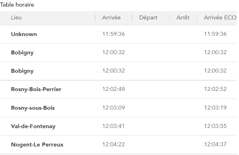
- The timetable for the passage of the train at the various points of interest.
3.1 - Physical modeling
Physical modelling plays an important role in the OSRD core calculation. It allows us to simulate train traffic, and it must be as realistic as possible train traffic, and it must be as realistic as possible.
Force review
To calculate the displacement of the train over time, we must first calculate its speed at each instant. A simple way to obtain this speed is to calculate the acceleration. Thanks to the fundamental principle of dynamics, the acceleration of the train at each instant is directly dependent on the different forces applied to it: $$ \sum \vec{F}=m\vec{a} $$
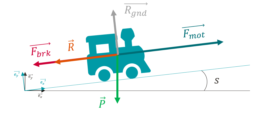
Traction: The value of the traction force \(F_{mot}\) depends on several factors:
- the rolling stock
- the speed of the train, \(v^{\prime}x\) according to the effort-speed curve below:
$$ {\vec{F_{mot}}(v_{x^{\prime}}, x^{\prime})=F_{mot}(v_{x^{\prime}}, x^{\prime})\vec{e_x^{\prime}}} $$

The x axis represents the speed of the train in [km/h], the y axis the value of the traction force in [kN].
- the action of the driver, who accelerates more or less strongly depending on where he is on his journey
- Braking : The value of the braking force \(F_{brk}\) also depends on the rolling stock and the driver’s action but has a constant value for a given rolling stock. In the current state of modelling, braking is either zero or at its maximum value.
$$ \vec{F_{brk}}(x^{\prime})=-F_{brk}(x^{\prime}){\vec{e_{x^{\prime}}}} $$
A second approach to modelling braking is the so-called hourly approach, as it is used for hourly production at SNCF. In this case, the deceleration is fixed and the braking no longer depends on the different forces applied to the train. Typical deceleration values range from 0.4 to 0.7m/s².
- Forward resistance: To model the forward resistance of the train, the Davis formula is used, which takes into account all the friction and aerodynamic resistance of the air. The value of the drag depends on the speed \(v^{\prime}_x\). The coefficients \(A\), \(B\), et \(C\) depend on the rolling stock.
$$ {\vec{R}(v_{x^{\prime}})}=-(A+Bv_{x^{\prime}}+{Cv_{x^{\prime}}}^2){\vec{e_{x^{\prime}}}} $$
- Weight (slopes + turns) : The weight force given by the product between the mass \(m\) of the train and the gravitational constant \(g\) is projected on the axes \(\vec{e_x}^{\prime}\) and \(\vec{e_y}^{\prime}\).For projection, we use the angle \(i(x^{\prime})\), which is calculated from the slope angle \(s(x^{\prime})\) corrected by a factor that takes into account the effect of the turning radius \(r(x^{\prime})\).
$$ \vec{P(x^{\prime})}=-mg\vec{e_y}(x^{\prime})= -mg\Big[sin\big(i(x^{\prime})\big){\vec{e_{x^{\prime}}}(x^{\prime})}+cos\big(i(x^{\prime})\big){\vec{e_{{\prime}}}(x^{\prime})}\Big] $$
$$ i(x^{\prime})= s(x^{\prime})+\frac{800m}{r(x^{\prime})} $$
- Ground Reaction : The ground reaction force simply compensates for the vertical component of the weight, but has no impact on the dynamics of the train as it has no component along the axis \({\vec{e_x}^{\prime}}\).
$$ \vec{R_{gnd}}=R_{gnd}{\vec{e_{y^{\prime}}}} $$
Forces balance
The equation of the fundamental principle of dynamics projected onto the axis \({\vec{e_x}^{\prime}}\) (in the train frame of reference) gives the following scalar equation:
$$ a_{x^{\prime}}(t) = \frac{1}{m}\Big [F_{mot}(v_{x^{\prime}}, x^{\prime})-F_{brk}(x^{\prime})-(A+Bv_{x^{\prime}}+{Cv_{x^{\prime}}}^2)-mgsin(i(x^{\prime}))\Big] $$
This is then simplified by considering that despite the gradient the train moves on a plane and by amalgamating \(\vec{e_x}\) and \(\vec{e_x}^{\prime}\). The gradient still has an impact on the force balance, but it is assumed that the train is only moving horizontally, which gives the following simplified equation:
$$ a_{x}(t) = \frac{1}{m}\Big[F_{mot}(v_{x}, x)-F_{brk}(x)-(A+Bv_{x}+{Cv_{x}}^2)-mgsin(i(x))\Big] $$
Resolution
The driving force and the braking force depend on the driver’s action (he decides to accelerate or brake more or less strongly depending on the situation). This dependence is reflected in the dependence of these two forces on the position of the train. The weight component is also dependent on the position of the train, as it comes directly from the slopes and bends below the train.
In addition, the driving force depends on the speed of the train (according to the speed effort curve) as does the resistance to forward motion. resistance.
These different dependencies make it impossible to solve this equation analytically, and the acceleration of the train at each moment must be calculated by numerical integration.
3.2 - Numerical integration
Introduction
Since physical modelling has shown that the acceleration of the train is influenced by various factors that vary along the route (gradient, curvature, engine traction force, etc.), the calculation must be carried out using a numerical integration method. The path is then separated into sufficiently short steps to consider all these factors as constant, which allows this time to use the equation of motion to calculate the displacement and speed of the train.
Euler’s method of numerical integration is the simplest way of doing this, but it has a number of drawbacks. This article explains the Euler method, why it is not suitable for OSRD purposes and which integration method should be used instead.
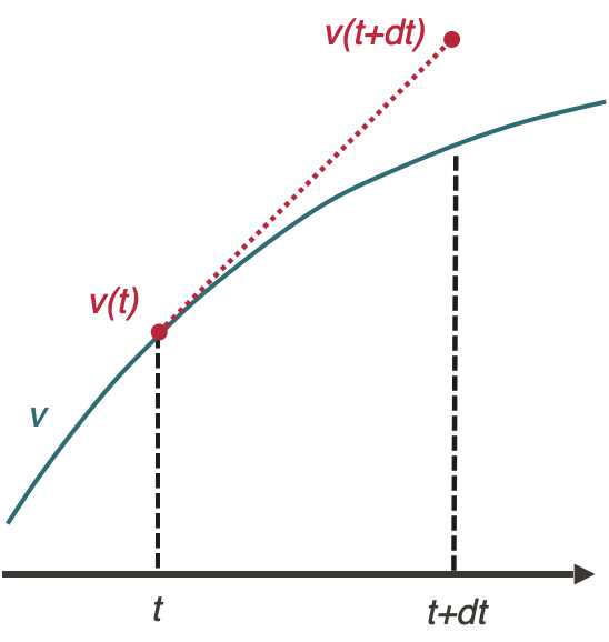
Euler’s method
The Euler method applied to the integration of the equation of motion of a train is:
$$v(t+dt) = a(v(t), x(t))dt + v(t)$$
$$x(t+dt) = \frac{1}{2}a(v(t), x(t))dt^2 + v(t)dt + x(t)$$
Advantages of Euler’s method
The advantages of the Euler method are that it is very simple to implement and has a rather fast calculation for a given time step, compared to other numerical integration methods (see appendix)
Disadvantages of the Euler’s method
The Euler integration method presents a number of problems for OSRD:
- It is relatively imprecise, and therefore requires a small time step, which generates a lot of data.
- With time integration, only the conditions at the starting point of the integration step (gradient, infrastructure parameters, etc.) are known, as one cannot predict precisely where it will end.
- We cannot anticipate future changes in the directive: the train only reacts by comparing its current state with its set point at the same time. To illustrate, it is as if the driver is unable to see ahead, whereas in reality he anticipates according to the signals, slopes and bends he sees ahead.
Runge-Kutta’s 4 method
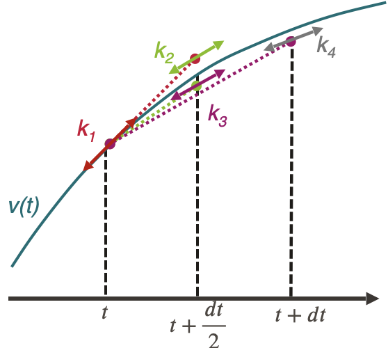
The Runge-Kutta 4 method applied to the integration of the equation of motion of a train is:
$$v(t+dt) = v(t) + \frac{1}{6}(k_1 + 2k_2 + 2k_3 + k_4)dt$$
With:
$$k_1 = a(v(t), x(t))$$
$$k_2 = a\Big(v(t+k_1\frac{dt}{2}), x(t) + v(t)\frac{dt}{2} + k_1\frac{dt^2}{8}\Big)$$
$$k_3 = a\Big(v(t+k_2\frac{dt}{2}), x(t) + v(t)\frac{dt}{2} + k_2\frac{dt^2}{8}\Big)$$
$$k_4 = a\Big(v(t+k_3dt), x(t) + v(t)dt + k_3\frac{dt^2}{2}\Big)$$
Advantages of Runge Kutta’s 4 method
Runge Kutta’s method of integration 4 addresses the various problems raised by Euler’s method:
- It allows the anticipation of directive changes within a calculation step, thus representing more accurately the reality of driving a train.
- It is more accurate for the same calculation time (see appendix), allowing for larger integration steps and therefore fewer data points.
Disadvantages of Runge Kutta’s 4 method
The only notable drawback of the Runge Kutta 4 method encountered so far is its difficulty of implementation.
The choice of integration method for OSRD
Study of accuracy and speed of calculation
Different integration methods could have replaced the basic Euler integration in the OSRD algorithm. In order to decide which method would be most suitable, a study of the accuracy and computational speed of different methods was carried out. This study compared the following methods:
- Euler
- Euler-Cauchy
- Runge-Kutta 4
- Adams 2
- Adams 3
All explanations of these methods can be found (in French) in this document, and the python code used for the simulation is here.
The simulation calculates the position and speed of a high-speed train accelerating on a flat straight line.
Equivalent time step simulations
A reference curve was simulated using the Euler method with a time step of 0.1s, then the same path was simulated using the other methods with a time step of 1s. It is then possible to simply compare each curve to the reference curve, by calculating the absolute value of the difference at each calculated point. The resulting absolute error of the train’s position over its distance travelled is as follows:
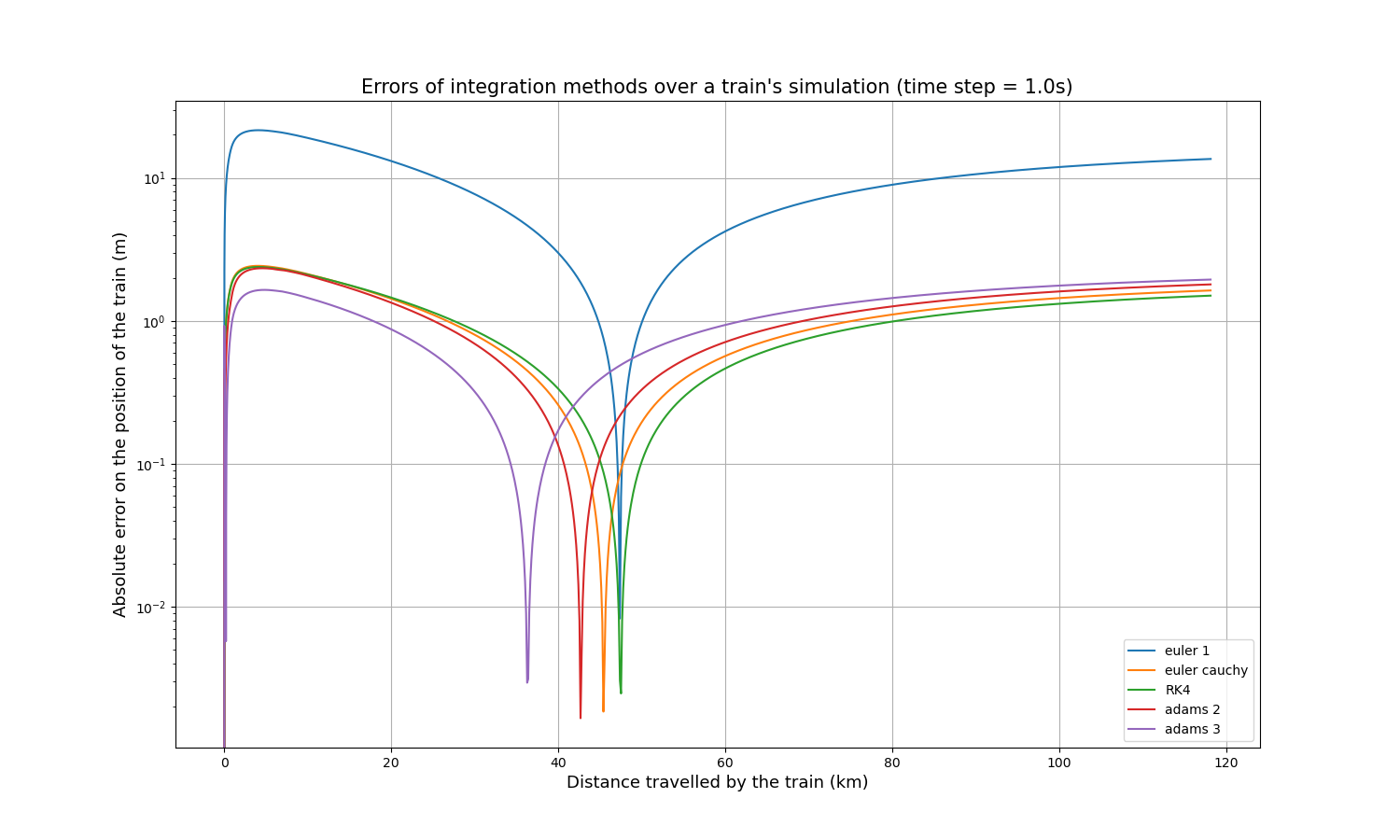
It is immediately apparent that the Euler method is less accurate than the other four by about an order of magnitude. Each curve has a peak where the accuracy is extremely high (extremely low error), which is explained by the fact that all curves start slightly above the reference curve, cross it at one point and end slightly below it, or vice versa.
As accuracy is not the only important indicator, the calculation time of each method was measured. This is what we get for the same input parameters:
| Integration method | Calculation time (s) |
|---|---|
| Euler | 1.86 |
| Euler-Cauchy | 3.80 |
| Runge-Kutta 4 | 7.01 |
| Adams 2 | 3.43 |
| Adams 3 | 5.27 |
Thus, Euler-Cauchy and Adams 2 are about twice as slow as Euler, Adams 3 is about three times as slow, and RK4 is about four times as slow. These results have been verified on much longer simulations, and the different ratios are maintained.
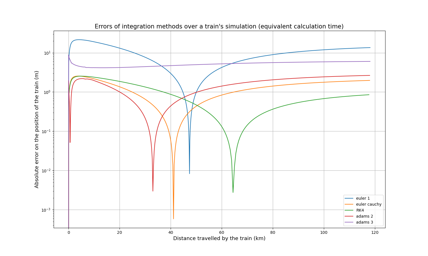
Simulation with equivalent calculation time
As the computation times of all methods depend linearly on the time step, it is relatively simple to compare the accuracy for approximately the same computation time. Multiplying the time step of Euler-Cauchy and Adams 2 by 2, the time step of Adams 3 by 3, and the time step of RK4 by 4, here are the resulting absolute error curves:
And here are the calculation times:
| Integration method | Calculation time (s) |
|---|---|
| Euler | 1.75 |
| Euler-Cauchy | 2.10 |
| Runge-Kutta 4 | 1.95 |
| Adams 2 | 1.91 |
| Adams 3 | 1.99 |
After some time, RK4 tends to be the most accurate method, slightly more accurate than Euler-Cauchy, and still much more accurate than the Euler method.
Conclusions of the study
The study of accuracy and computational speed presented above shows that RK4 and Euler-Cauchy would be good candidates to replace the Euler algorithm in OSRD: both are fast, accurate, and could replace the Euler method without requiring large implementation changes because they only compute within the current time step. It was decided that OSRD would use the Runge-Kutta 4 method because it is slightly more accurate than Euler-Cauchy and it is a well-known method for this type of calculation, so it is very suitable for an open-source simulator.
3.3 - Envelopes system
The envelope system is an interface created specifically for the OSRD gait calculation. It allows you to manipulate different space/velocity curves, to slice them, to end them, to interpolate specific points, and to address many other needs necessary for the gait calculation.
A specific interface in the OSRD Core service
The envelope system is part of the core service of OSRD (see software architecture).
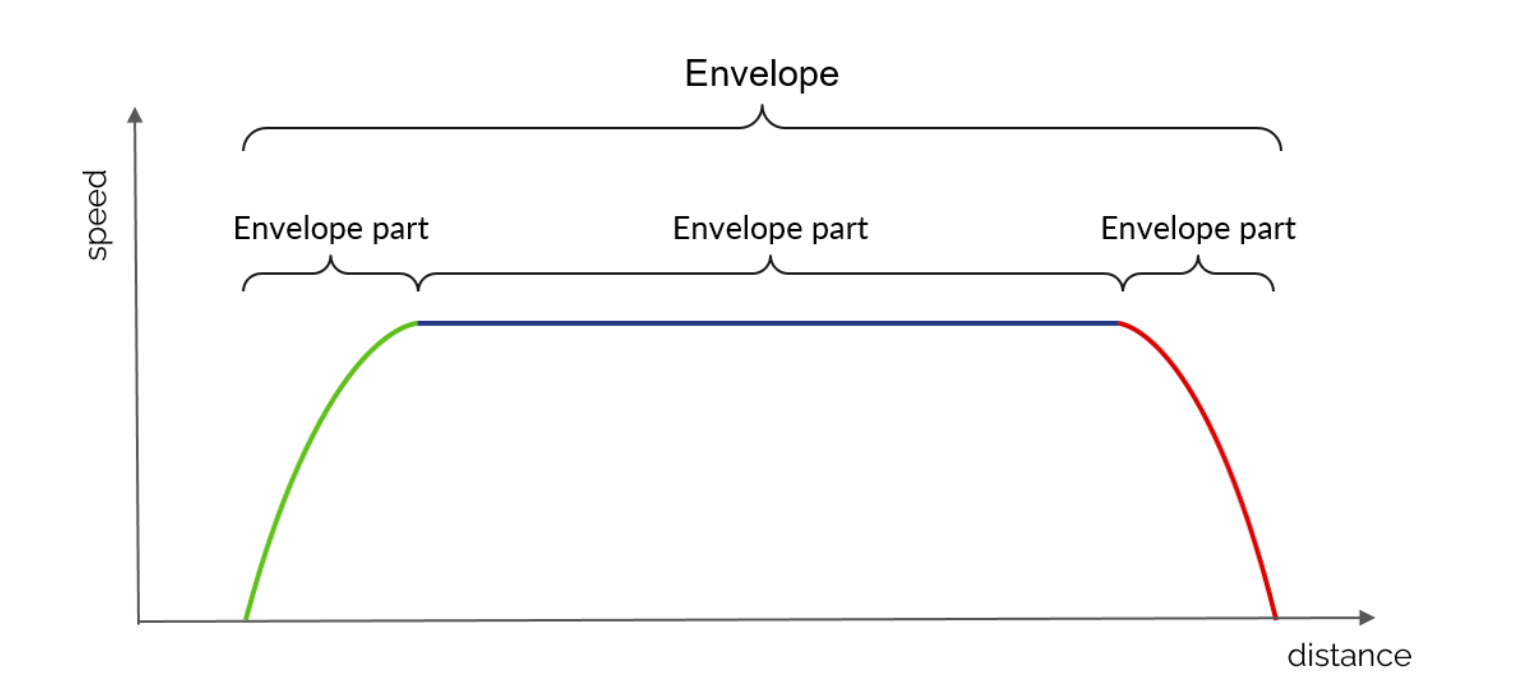
Its main components are :
1 - EnvelopePart: space/speed curve, defined as a sequence of points and having metadata indicating for example if it is an acceleration curve, a braking curve, a speed hold curve, etc.
2 - Envelope: a list of end-to-end EnvelopeParts on which it is possible to perform certain operations:
- check for continuity in space (mandatory) and speed (optional)
- look for the minimum and/or maximum speed of the envelope
- cut a part of the envelope between two points in space
- perform a velocity interpolation at a certain position
- calculate the elapsed time between two positions in the envelope
3 - Overlays : system for adding more constrained (i.e. lower speed) EnvelopeParts to an existing envelope.
Given envelopes vs. calculated envelopes
During the simulation, the train is supposed to follow certain speed instructions. These are modelled in OSRD by envelopes in the form of space/speed curves. Two types can be distinguished:
- Envelopes from infrastructure and rolling stock data, such as maximum line speed and maximum train speed. Being input data for our calculation, they do not correspond to curves with a physical meaning, as they are not derived from the results of a real integration of the physical equations of motion.
- The envelopes result from real integration of the physical equations of motion. They correspond to a curve that is physically tenable by the train and also contain time information.
A simple example to illustrate this difference: if we simulate a TER journey on a mountain line, one of the input data will be a maximum speed envelope of 160km/h, corresponding to the maximum speed of our TER. However, this envelope does not correspond to a physical reality, as it is possible that on certain sections the gradient is too steep for the train to be able to maintain this maximum speed of 160km/h. The calculated envelope will therefore show in this example a speed drop in the steepest areas, where the envelope given was perfectly flat.
Simulation of several trains
In the case of the simulation of many trains, the signalling system must ensure safety. The effect of signalling on the running calculation of a train is reproduced by superimposing dynamic envelopes on the static envelope. A new dynamic envelope is introduced for example when a signal closes. The train follows the static economic envelope superimposed on the dynamic envelopes, if any. In this simulation mode, a time check is performed against a theoretical time from the time information of the static economic envelope. If the train is late with respect to the scheduled time, it stops following the economic envelope and tries to go faster. Its space/speed curve will therefore be limited by the maximum effort envelope.
3.4 - Pipeline
The walk calculation in OSRD is a 4-step process, each using the envelopes system:
- Construction of the most restrictive speed profile
- Addition of the different braking curves
- Adding the different acceleration curves and checking the constant speed curves
- Application of allowance(s)
Calculation of the Most Restricted Speed Profile (MRSP)
A first envelope is calculated at the beginning of the simulation by grouping all static velocity limits:
- maximum line speed
- maximum speed of rolling stock
- temporary speed limits (e.g. in case of works on a line)
- speed limits by train category
- speed limits according to train load
- speed limits corresponding to signposts
The length of the train is also taken into account to ensure that the train does not accelerate until its tail leaves the slowest speed zone. An offset is then applied to the red dashed curve. The resulting envelope (black curve) is called the Most Restricted Speed Profile (MRSP). It is on this envelope that the following steps will be calculated.
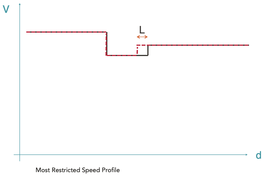
The red dotted line represents the maximum permitted speed depending on the position. The black line represents the MRSP where the train length has been taken into account.
It should be noted that the different envelopeParts composing the MRSP are input data, so they do not correspond to curves with a physical reality.
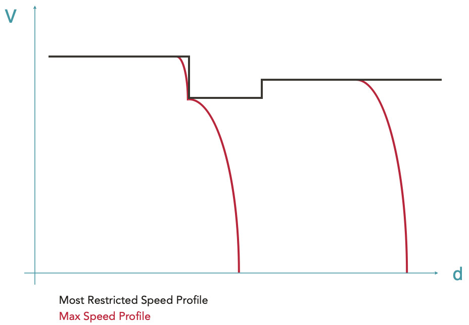
Calculation of the Max Speed Profile
Starting from the MRSP, all braking curves are calculated using the overlay system (see here for more details on overlays), i.e. by creating envelopeParts which will be more restrictive than the MRSP. The resulting curve is called Max Speed Profile. This is the maximum speed envelope of the train, taking into account its braking capabilities.
Since braking curves have an imposed end point and the braking equation has no analytical solution, it is impossible to predict their starting point. The braking curves are therefore calculated backwards from their target point, i.e. the point in space where a certain speed limit is imposed (finite target speed) or the stopping point (zero target speed).
For historical reasons in hourly production, braking curves are calculated at SNCF with a fixed deceleration, the so-called hourly deceleration (typically ~0.5m/s²) without taking into account the other forces. This method has therefore also been implemented in OSRD, allowing the calculation of braking in two different ways: with this hourly rate or with a braking force that is simply added to the other forces.
Calculation of the Max Effort Profile
For each point corresponding to an increase in speed in the MRSP or at the end of a stop braking curve, an acceleration curve is calculated. The acceleration curves are calculated taking into account all active forces (traction force, driving resistance, weight) and therefore have a physical meaning.
For envelopeParts whose physical meaning has not yet been verified (which at this stage are the constant speed running phases, always coming from the MRSP), a new integration of the equations of motion is performed. This last calculation is necessary to take into account possible speed stalls in case the train is physically unable to hold its speed, typically in the presence of steep ramps (see this example).
The envelope that results from the addition of the acceleration curves and the verification of the speed plates is called the Max Effort Profile.
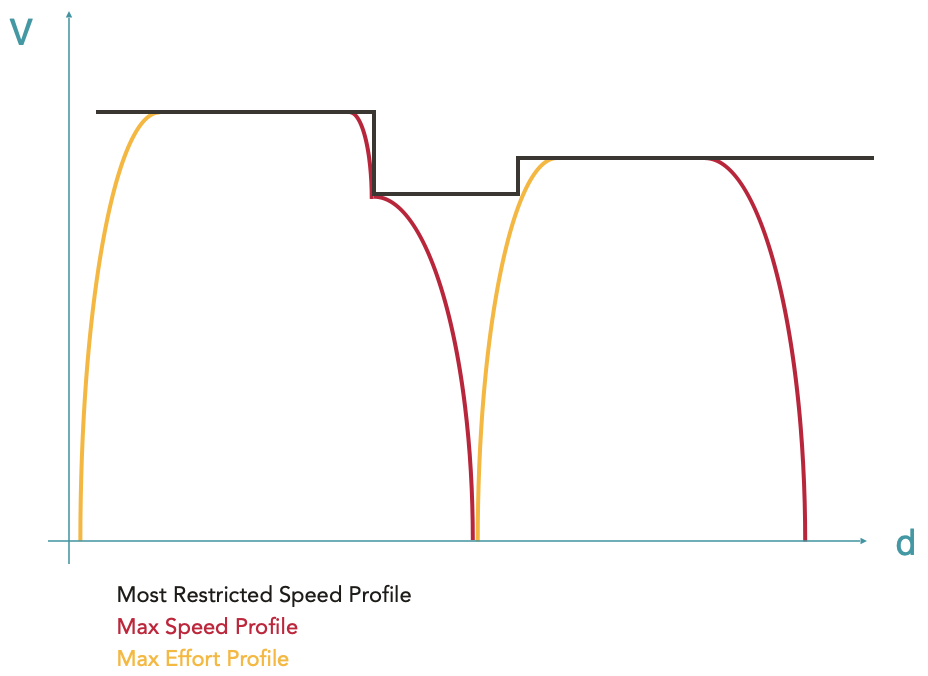
At this stage, the resulting envelope is continuous and has a physical meaning from start to finish. The train accelerates to the maximum, runs as fast as possible according to the different speed limits and driving capabilities, and brakes to the maximum. The resulting travel calculation is called the basic running time. It corresponds to the fastest possible route for the given rolling stock on the given route.
Application of allowance(s)
After the calculation of the basic run (corresponding to the Max Effort Profile in OSRD), it is possible to apply allowances. Allowances are additions of extra time to the train’s journey. They are used to allow the train to catch up if necessary or for other operational purposes (more details on allowances here).
A new Allowances envelope is therefore calculated using overlays to distribute the allowance requested by the user over the maximum effort envelope calculated previously.
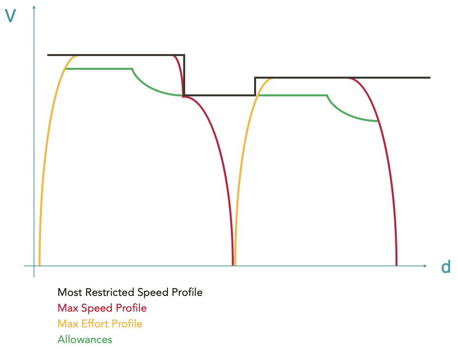
In the OSRD running calculation it is possible to distribute the allowances in a linear way, by lowering all speeds by a certain factor, or in an economic way, i.e. by minimising the energy consumption during the train run.
3.5 - Allowances
The purpose of allowances
As explained in the calculation of the Max Effort Profile, the basic running time represents the most stretched run normally achievable, i.e. the fastest possible run of the given equipment on the given route. The train accelerates to the maximum, travels as fast as possible according to the different speed limits and driving capabilities, and brakes to the maximum.
This basic run has a major disadvantage: if a train leaves 10 minutes late, it will arrive at best 10 minutes late, because by definition it is impossible for it to run faster than the basic run. Therefore, trains are scheduled with one or more allowances added. The allowances are a relaxation of the train’s route, an addition of time to the scheduled timetable, which inevitably results in a lowering of running speeds.
A train running in basic gear is unable to catch up!
Allowances types
There are two types of allowances:
- The regularity allowance: this is the additional time added to the basic running time to take account of the inaccuracy of speed measurement, to compensate for the consequences of external incidents that disrupt the theoretical run of trains, and to maintain the regularity of the traffic. The regularity allowance applies to the whole route, although its value may change at certain intervals.
- The construction allowance: this is the time added/removed on a specific interval, in addition to the regularity allowance, but this time for operational reasons (dodging another train, clearing a track more quickly, etc.)
A basic running time with an added allowance of regularity gives what is known as a standard walk.
Allowance distribution
Since the addition of allowance results in lower speeds along the route, there are a number of possible routes. Indeed, there are an infinite number of solutions that result in the same journey time.
As a simple example, in order to reduce the running time of a train by 10% of its journey time, it is possible to extend any stop by the time equivalent to this 10%, just as it is possible to run at 1/1.1 = 90.9% of the train’s capacity over the entire route, or to run slower, but only at high speeds…
There are currently two algorithms for margin distribution in OSRD: linear and economic.
Linear distribution
Linear allowance distribution is simply lowering the speeds by the same factor over the area where the user applies the allowance. Here is an example of its application:
The advantage of this distribution is that the allowance is spread evenly over the entire journey. A train that is late on 30% of its journey will have 70% of its allowance for the remaining 70% of its journey.
Economic distribution
The economic distribution of the allowance, presented in detail in this document (MARECO is an algorithm designed by the SNCF research department), consists of distributing the allowance in the most energy-efficient way possible. It is based on two principles:
- a maximum speed, avoiding the most energy-intensive speeds
- run-on zones, located before braking and steep gradients, where the train runs with the engine off thanks to its inertia, allowing it to consume no energy during this period
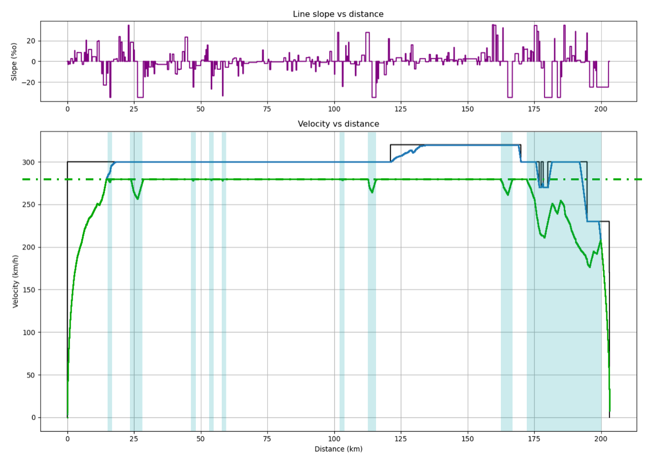
An example of economic walking. Above, the gradients/ramps encountered by the train. The areas of travel on the track are shown in blue.
4 - Netzgrafik-Editor
Open-source software developed by SBB CFF FFS and its integration in OSRD
Netzgrafik-Editor (NGE) is an open-source software that enables the creation, modification, and analysis of regular-interval timetable, at a macroscopic level of detail, developed by Swiss Federal Railways (SBB CFF FFS). See front-end and back-end repositories.
OSRD and NGE are are semantically different: the former uses a microscopic level of detail, based on a well-defined infrastructure, depicting a timetable composed of unique train schedules, while the latter uses a macroscopic level of detail, not based on any explicit infrastructure, depicting a transportation plan made up of regular-interval based train runs. However, these differences, close enough, may be arranged to make it work together.
The compatibility between NGE and OSRD has been tested through a proof of concept, by running both pieces of software as separate services and without automated synchronization.
The idea is to give to OSRD a graphical tool to edit (create, update and delete train schedules from) a timetable from an operational study scenario, and get some insights on analytics at the same time. Using both microscopic and macroscopic levels of detail brings a second benefit: OSRD’s microscopic calculations extend the actual scope of NGE, its functionalities and information provided, such as the microscopic simulations or the conflicts detection tool.
The transversal objective of this feature is to make two open-source projects from two big railway infrastructure managers work along and cooperate with one another with the same goal: ensure a digital continuity on different time scales for railway operational studies.
1 - Integration in OSRD
OSRD has developed a standalone version of NGE, integrated into the source code, which allows NGE to work without a back-end. Thus, for external use, a build of NGE standalone is available on NPM and is published at each release. Finally, to meet OSRD-specific needs, OSRD uses a fork of NGE (whose build, NGE standalone, is also available on NPM), remaining as close as possible to the official directory.
Despite using different JavaScript frameworks (ReactJS for OSRD and Angular for NGE), this build allows OSRD to integrate NGE within an iframe. This iframe instantiates a Custom Element, which is be the communication interface between both applications and launch NGE’s build.
An alternative solution to the integration problem would have been to rewrite NGE as web-components, in order to import them into OSRD, but this solution was abandoned because of the amount of work it would represent.
NGE, in its standalone version, communicates with OSRD through the iframe using DOM element properties:
@Input: with thenetzgrafikDtoproperty, triggered when the content of the scenario is updated from OSRD.@Output: with theoperationsproperty, triggered when NGE is used.
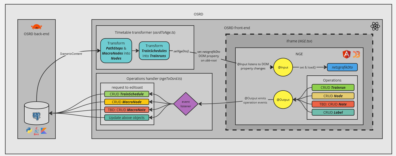
NGE is then able to obtain the OSRD timetable as soon as a change is made on the OSRD side, and OSRD is able to obtain the changes made on the NGE side.
2 - Converters
To overcome semantic differences and adapt data models, two converters are implemented:
- [OSRD -> NGE] a converter which transforms an OSRD timetable into an NGE model. The nodes are the waypoints described by the train schedules, and whose macroscopic information (position on the reticular) is stored in the database. OSRD train schedules,
TrainSchedule, then represent cadenced train lines in NGE,Trainrun. A concept of cadenced train lines, will soon be implemented to allow conceptual convergence between OSRD and NGE. - [OSRD <- NGE] an event manager, which transforms an NGE action into an update of the OSRD database.
3 - Open-source (cooperation / contribution)
To make NGE compatible with OSRD, some changes have been requested (disable back-end, create hooks on events) and directly implemented in the official repository of NGE, with the agreement and help of NGE team.
Contributions for one project to another, from both sides, are valuable and will be entertained in the future.
This feature also shows that open-source cooperation is powerful and a huge gain of time in software development.