Whether you would like to use OSRD, understand it or contribute, this is the right place!
This is the multi-page printable view of this section. Click here to print.
Documentation
- 1: Explanations
- 1.1: Containers architecture
- 1.2: Models
- 1.2.1: Infrastructure example
- 1.2.2: Neutral Sections
- 1.2.3: Rolling stock categories
- 1.3: Running time calculation
- 1.3.1: Physical modeling
- 1.3.2: Numerical integration
- 1.3.3: Envelopes system
- 1.3.4: Pipeline
- 1.3.5: Allowances
- 1.4: Netzgrafik-Editor
- 2: How-to Guides
- 2.1: Contribute to OSRD
- 2.1.1: Preamble
- 2.1.2: License and set-up
- 2.1.3: Contribute code
- 2.1.3.1: General principles
- 2.1.3.2: Back-end conventions
- 2.1.3.3: Front-end conventions
- 2.1.3.4: Write code
- 2.1.3.5: Commit conventions
- 2.1.3.6: Share your changes
- 2.1.3.7: Tests
- 2.1.4: Review process
- 2.1.5: Report issues
- 2.1.6: Install docker
- 2.1.7:
- 2.2: Deploy OSRD
- 2.2.1: Docker Compose
- 2.2.2: Kubernetes with Helm
- 2.2.3: STDCM search environment configuration
- 2.3: Logo
- 2.4: OSRD's design
- 2.5: Release
- 2.5.1: Release process
- 2.5.2: Publish a new release
- 3: Technical reference
- 3.1: Architecture
- 3.2: Design documents
- 3.2.1: Interlocking
- 3.2.2: Signaling
- 3.2.2.1: Signaling systems
- 3.2.2.2: Blocks and signals
- 3.2.2.3: Speed limits
- 3.2.2.4: Simulation lifecycle
- 3.2.3: Conflict detection
- 3.2.4: Train simulation v3
- 3.2.4.1: Overview
- 3.2.4.2: Prior art
- 3.2.4.3: Driving instructions
- 3.2.4.4: Driver behavior modules
- 3.2.5: Search for last-minute train slots (STDCM)
- 3.2.5.1: Business context
- 3.2.5.2: Train slot search module
- 3.2.5.2.1: Infrastructure exploration
- 3.2.5.2.2: Conflict detection
- 3.2.5.2.3: Conflict avoidance
- 3.2.5.2.4: Discontinuities and backtracking
- 3.2.5.2.5: Search space and decision tree
- 3.2.5.2.6: The actual pathfinding
- 3.2.5.2.7: Standard allowance
- 3.2.5.2.8: Implementation details and current issues
- 3.2.6: Timetable v2
- 3.2.7: Authentication and authorization
- 3.2.7.1: Editoast internal authorization API
- 3.2.8: Editoast error management
- 3.2.9: Scalable async RPC
- 3.3: APIs
- 3.3.1: Editoast
- 3.3.2: Gateway
- 3.3.3: Railway Manager Interface
- 4: Railway Wiki
- 4.1: Glossary
- 4.2: Signalling
- 4.2.1: Railway risks
- 4.2.2: Signals
- 4.2.3: Line operation modes
- 4.2.3.1: Single-track lines
- 4.2.3.2: Double-track lines
- 4.2.4: Train spacing systems
- 4.2.4.1: Automatic block systems
- 4.2.4.2: ETCS (ERTMS)
- 4.2.4.2.1: ETCS
- 4.2.4.3: Ks Signalling
- 4.2.4.3.1: Linienförmige Zugbeeinflussung (LZB)
- 4.2.4.3.2: Punktförmige Zugbeeinflussung (PZB)
1 - Explanations
Learn more about key concepts
Explanations discuss key topics and concepts at a fairly high level and provide useful background information and explanation.
1.1 - Containers architecture
How the containers works together and how they are built
There are 3 main containers deployed in a standard OSRD setup:
- Gateway (includes the frontend): Serves the front end, handles authentication and proxies requests to the backend.
- Editoast: Acts as the backend that interacts with the front end.
- Core: Handles computation and business logic, called by Editoast.
Standard deployment
The standard deployment can be represented with the following diagram.
flowchart TD
    gw["gateway"]
    front["front-end static files"]
    gw -- local file --> front

    browser --> gw
    gw -- HTTP --> editoast
    editoast -- HTTP --> core
External requests are received by the gateway. If the path asked starts with /api it will be forwarded using HTTP to editoast, otherwise it will serve a file with the asked path. Editoast reach the core using HTTP if required.
The gateway is not only a reverse proxy with the front-end bundle included, it also provides all the authentication mechanisms: using OIDC or tokens.
1.2 - Models
What is modeled in OSRD, and how it is modeled
1.2.1 - Infrastructure example
Explains using an example how infrastructure data is structured
Introduction
This page gives an example of how the data formats are used to describe an infrastructure in OSRD.
For this purpose, let’s take as an example the following toy infrastructure:

Tip
To zoom in on diagrams, click on the edit button that appears when hovering over it.This diagram is an overview of the infrastructure with lines and stations only.
This infrastructure is not meant to be realistic, but rather meant to help illustrate OSRD’s data model. This example will be created step by step and explained along the way.
The infrastructure generator
In the OSRD repository is a python library designed to help generate infrastructures in a format understood by OSRD.
The infrastructure discussed in this section can be generated thanks to small_infra.py file. To learn more about the generation scripts, you can check out the related README.
Tracks
Track sections
The first objects we need to define are TrackSections. Most other objects are positioned relative to track sections.
A track section is a section of rail (switches not included). One can chose to divide the tracks of their infrastructure in as many track sections as they like. Here we chose to use the longest track sections possible, which means that between two switches there is always a single track section.
Track sections is what simulated trains roll onto. They are the abstract equivalent to physical rail sections. Track sections are bidirectional.
In this example, we define two tracks for the line between the West and North-East stations. We also have overpassing tracks at the North and Mid-West stations for added realism. Finally, we have three separate tracks in the West station, since it’s a major hub in our imaginary infrastructure.

Important
TrackSections are represented as arrows in this diagram to stress the fact that they have a start and an end. It matters as objects positioned on track sections are located using their distance from the start of their track section.
Therefore, to locate an object at the beginning of its track section, set its offset to 0. To move it to the end of its track section, set its offset to the length of the track section.
These attributes are required for the track section to be complete:
length: the length of the track section in meters.geo: the coordinates in real life (geo is for geographic), in the GeoJSON format.- cosmetic attributes:
line_name,track_name,track_numberwhich are used to indicate the name and labels that were given to the tracks / lines in real life.
For all track sections in our infrastructure, the geo attributes very much resemble the given diagram.
For most track sections, their length is proportional to what can be seen in the diagram. To preserve readability, exceptions were made for TA6, TA7, TD0 and TD1 (which are 10km and 25km).
Node
A Node represents a node in the infrastructure. In an OSRD simulation, a train can only move from one section of track to another if they are linked by a node.
Node Types
NodeTypes have two mandatory attributes:
ports: A list of port names. A port is an endpoint connected to a track section.groups: A mapping between group names and lists of branch (connection between 2 ports) that characterises the different possible positions of the node type
At any time, all nodes have an active group, and may have an active branch, which always belongs to the active group. During a simulation, changing the active branch inside a group is instantaneous, but changing the active branch across groups (changing the active group) takes configurable time.
This is because a node is a physical object, and changing active branch can involve moving parts of it. Groups are designed to represent the different positions that a node can have. Each group contains the branches that can be used in the associated node position.
The duration needed to change group is stored inside the Node, since it can vary depending on the physical implementation of the node.
Our examples currently use five node types. Node types are just like other objects, and can easily be added as needed using extended_switch_type.
1) Link
This one represents the link between two sections of track. It has two ports: A and B.

It is used in the OSRD model to create a link between two track sections. This is not a physical object.
2) The Point Switch
The ubiquitous Y switch, which can be thought of as either two tracks merging, or one track splitting.
This node type has three ports: A, B1 and B2.

There are two groups, each with one connection in their list: A_B1, which connects A to B1, and A_B2 which connects A to B2.
Thus, at any given moment (except when the switch moves from one group to another), a train can go from A to B1 or from A to B2 but never to both at the same time. A train cannot go from B1 to B2.
A Point Switch only has two positions:
- A to B1
- A to B2


3) The Crossing
This is simply two tracks crossing each other.
This type has four ports: A1, B1, A2 et B2.

It has only one group containing two connections: A1 to B1 and A2 to B2. Indeed this kind of switch is passive: it has no moving parts. Despite having a single group, it is still used by the simulation to enforce route reservations.
Here are the two different connections this switch type has:
- A1 to B1
- A2 to B2


4) The Double slip switch
This one is more like two point switches back to back. It has four ports: A1, A2, B1 and B2.

However, it has four groups, each with one connection. The four groups are represented in the following diagram:
- A1 to B1
- A1 to B2
- A2 to B1
- A2 to B2


5) The Single slip switch
This one looks more like a cross between a single needle and a crossover. It has four ports: A1, A2, B1 and B2.

Here are the three connections that can be made by this switch:
- A1 to B1
- A1 to B2
- A2 to B2


Back to nodes
A Node has three attributes:
node_type: the identifier of theNodeTypeof this node.ports: a mapping from port names to track sections extremities.group_change_delay: the time it takes to change which group of the node is activated.
The port names must match the ports of the node type chosen. The track section endpoints can be start or end, be careful to chose the appropriate ones.
Most of our example’s nodes are regular point switches. The path from North station to South station has two cross switches. Finally, there is a double cross switch right before the main line splits into the North-East and South-East lines.

It is important to note that these node types are hard-coded into the project code. Only the extended_node_type added by the user will appear in the railjson.
Curves and slopes
Curves and Slopes are instrumental to realistic simulations. These objects are defined as a range between a begin and end offsets of one track section. If a curve / slope spans more than one track section, it has to be added to all of them.
The slope / curve values are constant on their entire range. For varying curves / slopes, one needs to create several objects.
Slope values are measured in meters per kilometers, and the curve values are measured in meters (the radius of the curve).
Mind that the
begin value should always be smaller than the end value. That is why the curve / slope values can be negative: an uphill slope of 1 going from offset 10 to 0 is the same as a downhill slope of -1 going from offsets 0 to 10.In the small_infra.py file, we have slopes on the track sections TA6, TA7, TD0 and TD1.
There are curves as well, on the track sections TE0, TE1, TE3 and TF1.
Interlocking
All objects so far contributed to track topology (shape). Topology would be enough for trains to navigate the network, but not enough to do so safely. To ensure safety, two systems collaborate:
- Interlocking ensures trains are allowed to move forward
- Signaling is the mean by which interlocking communicates with the train
Detectors
These objects are used to create TVD sections (Track Vacancy Detection section): the track area in between detectors is a TVD section. When a train runs into a detector, the section it is entering becomes occupied. The only function of TVD sections is to locate trains.
In real life, detectors can be axle counters or track circuits for example.
For this mean of location to be efficient, detectors need to be placed regularly along your tracks, not too many because of cost, but not too few, because then TVD sections would be very large and trains would need to be very far apart to be told apart, which reduces capacity.
There often are detectors close to all sides of switches. This way, interlocking is made aware pretty much immediately when a switch is cleared, which is then free to be used again.
Let’s take a cross switch as an example: if train A is crossing it north to south and train B is coming to cross west to east, then as soon as train A’s last car has passed the crossing, B should be able to go, since A is now on a completely unrelated track section.
In OSRD, detectors are point objects, so all the attributes it needs are its id, and track location (track and offset).

The clumped up squares represent many detectors at once. Indeed, because some track sections are not represented with their full length, we could not represent all the detectors on the corresponding track section.
Some notes:
- Between some points, we added only one detector (and not two), because they were really close together, and it would have made no sense to create a tiny TVDS between the two. This situation happened on track sections (TA3, TA4, TA5, TF0 and TG3).
- In our infrastructure, there are relatively few track sections which are long enough to require more detectors than just those related to switches. Namely, TA6, TA7, TDO, TD1, TF1, TG1 and TH1. For example TD0, which measures 25km, has in fact 17 detectors in total.
Buffer stops
BufferStops are obstacles designed to prevent trains from sliding off dead ends.
In our infrastructure, there is a buffer stop on each track section which has a loose end. There are therefore 8 buffer stops in total.
Together with detectors, they set the boundaries of TVD sections (see Detectors)
Routes
A Route is an itinerary in the infrastructure. A train path is a sequence of routes. Routes are used to reserve section of path with the interlocking. See the dedicated documentation.
It is represented with the following attributes:
entry_pointandexit_point: references detectors or buffer stops which mark the beginning and the end of the Route.entry_point_direction: Direction on a track section to start the route from theentry_point.switches_direction: A set of directions to follow when we encounter a switch on our Route, to build this Route fromentry_pointtoexit_point.release_detectors: When a train clears a release detector, resources reserved from the beginning of the route until this detector are released.
Signaling
Thanks to interlocking, trains are located and allowed to move. It’s a good start, but meaningless until trains are made aware of it. This is where Signals come into play: signals react to interlocking, and can be seen by trains.
How trains react to signals depends on the aspect, kind of signal, and signaling system.
Here are the most important attributes for signals:
linked_detector: The linked detector.type_code: The type of signal.direction: The direction it protects, which can simply be interpreted as the way in which it can be seen by an incoming train (since there are lights only on one side…). Direction is relative to track section orientation.- Cosmetic attributes like
angle_geoorsidewhich control the way in which the signals are displayed in the front-end.
Here is a visualization of how one can represent a signal, and which direction it protects.

The way the signals are arranged is highly dependent on both signaling system and infrastructure manager.
Here are the basic rules used for this example infrastructure:
- We add two spacing signals (one per direction) for each detector that is cutting a long TVD section into smaller ones.
- Switch entries where a train might have to stop are protected by a signal (which is located outside of the switch TVD section). It must be visible from the direction used to approach the switch. When there are multiple switches in a row, only the first one usually needs protection, as interlocking is usually designed as not to encourage trains stopping in the middle of intersections.
Note that detectors linked to at least one signal are not represented, as there are not signals without associated detectors in this example.
To get the id of a detector linked to a signal, take the signal’s id and replace S by D (e.g. SA0 -> DA0).

On TA6, TA7, TD0 and TD1 we could not represent all signals because these track sections are very long and have many detectors, hence many signals.
Electrification
To allow electric trains to run on our infrastructure, we need to specify which parts of the infrastructure is electrified.
Catenaries
Catenaries are objects that represent the overhead wires that power electric trains. They are represented with the following attributes:
voltage: A string representing the type of power supply used for electrificationtrack_ranges: A list of range of track sections (TrackRanges) covered by this catenary. ATrackRangeis composed of a track section id, abeginoffset and anendoffset.
In our example infrastructure, we have two Catenaries:
- One with
voltageset to"1500", which covers only TA0. - One with
voltageset to"25000", which covers all others except TD1.
This means that only thermal trains can cross the TD1 track section.
Our example also outlines that, unlike its real life counterpart, a single Catenary may cover the whole infrastructure.
Neutral Sections
In some parts of an infrastructure, the train drivers may be instructed - mainly for safety reasons - to cut the power supply to the train.
To represent such parts, we use NeutralSections. They are represented mainly with the following attributes:
track_ranges: A list ofDirectedTrackRanges(track ranges associated to a direction) which are covered by this neutral section.lower_pantograph: A boolean indicating whether the train’s pantograph should be lowered while in this section.
In our example infrastructure, we have three NeutralSections: one at the junction of the "1500" and "25000" catenaries, one on TA6 and one on TG1 and TG4.
For more details about the model see the dedicated page.
Miscellaneous
Operational points
Operational point is also known in French as “Point Remarquable” (PR).
One OperationalPoint is a collection of points (OperationalPointParts) of interest.
For example, it may be convenient (reference point for train operation) to store the location of platforms as parts and group them by station in operational points.
In the same way, a bridge over tracks will be one OperationalPoint, but it will have several OperationPointParts, one at the intersection of each track. The local_track_name field provides a human-friendly track label in the context of the operational point.
In the example infrastructure, we only used operational points to represent stations. Operational point parts are displayed as purple diamonds. Keep in mind a single operational point may contain multiple parts.

Loading Gauge Limits
These objects are akin to Slopes and Curves: it covers a range of track section, with a begin and an end offset. It represents a restriction on the trains that can travel on the given range, by weight or by train type (freight or passenger).
We did not put any in our examples.
Speed Sections
The SpeedSections represent speed limits (in meters per second) that are applied on some parts of the tracks. One SpeedSection can span on several track sections, and do not necessarily cover the whole track sections. Speed sections can overlap.
In our example infrastructure, we have a speed section covering the whole infrastructure, limiting the speed to 300 km/h. On a smaller part of the infrastructure, we applied more restrictive speed sections.

1.2.2 - Neutral Sections
Documentation about what they are and how they are implemented
Physical object to model
Introduction
For a train to be able to run, it must either have an energy source on board (fuel, battery, hydrogen, …) or be supplied with energy throughout its journey.
To supply this energy, electrical cables are suspended above the tracks: the catenaries. The train then makes contact with these cables thanks to a conducting piece mounted on a mechanical arm: the pantograph.
Neutral sections
With this system it is difficult to ensure the electrical supply of a train continuously over the entire length of a line. On certain sections of track, it is necessary to cut the electrical supply of the train. These portions are called neutral sections.
Indeed, in order to avoid energy losses along the catenaries, the current is supplied by several substations distributed along the tracks. Two portions of catenaries supplied by different substations must be electrically isolated to avoid short circuits.
Moreover, the way the tracks are electrified (DC or not for example) can change according to the local uses and the time of installation. It is again necessary to electrically isolate the portions of tracks which are electrified differently. The train must also (except in particular cases) change its pantograph when the type of electrification changes.
In both cases, the driver is instructed to cut the train’s traction, and sometimes even to lower the pantograph.
In the French infrastructure, these zones are indicated by announcement, execution and end signs. They also carry the indication to lower the pantograph or not. The portions of track between the execution and end may not be electrified entirely, and may not even have a catenary (in this case the zone necessarily requires lowering the pantograph).
REV (for reversible) signs are sometimes placed downstream of the end of zone signs. They are intended for trains that run with a pantograph at the rear of the train. These signs indicate that the driver can resume traction safely.
Additionally, it may sometimes be impossible on a short section of track to place a catenary or to raise the train’s pantograph. In this case the line is still considered electrified, and the area without electrification (passage under a bridge for example) is considered as a neutral section.
Rolling stock
After passing through a neutral section, a train must resume traction. This is not immediate (a few seconds), and the necessary duration depends on the rolling stock.
In addition, the driver must, if necessary, lower his pantograph, which also takes time (a few tens of seconds) and also depends on the rolling stock.
Thus, the coasting imposed on the train extends outside the neutral section, since these system times are to be counted from the end of the neutral section.
Data model
We have chosen to model the neutral sections as the space between the signs linked to it (and not as the precise zone where there is no catenary or where the catenary is not electrified).
This zone is directional, i.e. associated with a direction of travel, in order to be able to take into account different placements of signs according to the direction. The execution sign of a given direction is not necessarily placed at the same position as the end of zone sign of the opposite direction.
For a two-way track, a neutral section is therefore represented by two objects.
The schema is the following
{
    "lower_pantograph": boolean,
    "track_ranges": [
        {
            "track": string,
            "start": number,
            "end": number,
            "direction": enum
        }
    ],
    "announcement_track_ranges": [
        {
            "track": string,
            "start": number,
            "end": number,
            "direction": enum
        }
    ]
}
lower_pantograph: indicates whether the pantograph should be lowered in this sectiontrack_ranges: list of track sections ranges where the train must not tractionannouncement_track_ranges: list of track sections ranges between the announcement sign and the execution sign
Display
Map
The zones displayed in the map correspond to the track_ranges of neutral sections, thus are between the execution and end signs of the zone. The color of the zone indicates whether the train must lower its pantograph in the zone or not.
The direction in which the zone applies is not represented.
Simulation results
In the linear display, it is always the area between EXE and FIN that is displayed.
Pathfinding
Neutral sections are therefore portions of “non-electrified” track where an electric train can still run (but where it cannot traction).
When searching for a path in the infrastructure, an electric train can travel through a track section that is not covered by the track_ranges of a catenary object (documentation to be written) only if it is covered by the track_ranges of a neutral section.
Simulation
In our simulation, we approximate the driver’s behavior as follows:
- The coasting is started as soon as the train’s head passes the announcement sign
- The system times (pantograph reading and traction resumption) start as soon as the train’s head passes the end sign.
In the current simulation, it is easier to use spatial integration bounds rather than temporal ones. We make the following approximation: when leaving the neutral section, we multiply the system times by the speed at the exit of the zone. The coasting is then extended over the obtained distance. This approximation is reasonable because the train’s inertia and the almost absence of friction guarantee that the speed varies little over this time interval.
Improvements to be made
Several aspects could be improved:
- We do not model the REV signs, all trains therefore only have one pantograph at the front in our simulations.
- System times are approximated.
- The driver’s behavior is rather restrictive (coasting could start after the announcement sign).
- The display of the zones is limited: no representation of the direction or the announcement zones.
- These zones are not editable.
1.2.3 - Rolling stock categories
Defines rolling stock categories
Categories are groupings of rolling stock, either by their characteristics, performance or by the nature of the services for which they have been designed or are used.
The same rolling stock can be used for different types of operations and services. This versatility is reflected in the following attributes:
primary_category(required) indicates the main use of a rolling stockother_categories(optional) indicates other possible uses of a rolling stock
The primary category of a rolling stock enables several features, such as filtering, differentiated display on charts or network graphic views, and, more broadly, the aggregation of rolling stocks.
Categories of rolling stocks
The different default rolling stock categories are as follows:
High-speed train(see High-speed train)Intercity train(see Intercity train)Regional train(see Regional train)Commuter train(see Commuter train)Freight train(see Freight train)Fast freight train(same as Freight train, but with a different composition code,ME140instead ofMA100for example)Night train(see Night train)Tram-train(see Tram-train)Touristic train(see Touristic train)Work train(see Work train)
It is also planned that, in the future, a user will be able to create new rolling stock categories directly.
Realistic open data rolling stocks
To make the application more accessible to users outside the railway industry, such as external contributors and research laboratories, and to prepare for the release of the public playground version of OSRD, several rolling stock created with mock data are available to all users.
These rolling stocks are designed to cover most simulation scenarios that users may encounter.
These rolling stocks are not actual rolling stocks, due to confidentiality reasons, but they have been created based on real data to ensure a high level of realism.
The rolling stocks are provided as JSON files. We created one representative rolling stock for each category listed above.
The characteristics of these rolling stocks have been calculated based on the average values of real rolling stocks within each category. Additionally, most of these models are designed to be compatible across various networks: they are primarily bi-mode (supporting multiple electric voltage and current supply types), which is not always the case for real-world rolling stocks.
An example of rolling stock, a high-speed train, is represented below, from the rolling stock editor of the application:
Open data
Since these rolling stocks are fictional (yet realistic), they can be freely used in projects beyond OSRD.
To access and use them in the application:
From the open-source playground: The rolling stocks are available by default.
From a locally launched application: Use the corresponding command in the README to import the test rolling stocks in your database.
1.3 - Running time calculation
OSRD can be used to perform two types of calculations:
- Standalone train simulation: calculation of the travel time of a train on a given route without interaction between the train and the signalling system.
- Simulation: “dynamic” calculation of several trains interacting with each other via the signalling system.
1 - The input data
A running time calculation is based on 5 inputs:
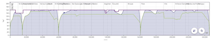
- Infrastructure: Line and track topology, position of stations and passenger buildings, position and type of points, signals, maximum line speeds, corrected line profile (gradients, ramps and curves).
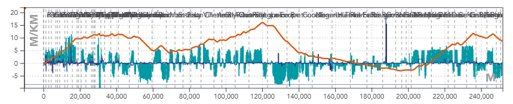
The blue histogram is a representation of the gradients in [‰] per position in [m]. The gradients are positive for ramps and negative for slopes.
The orange line represents the cumulative profile, i.e. the relative altitude to the starting point.
The blue line is a representation of turns in terms of radii of curves in [m].
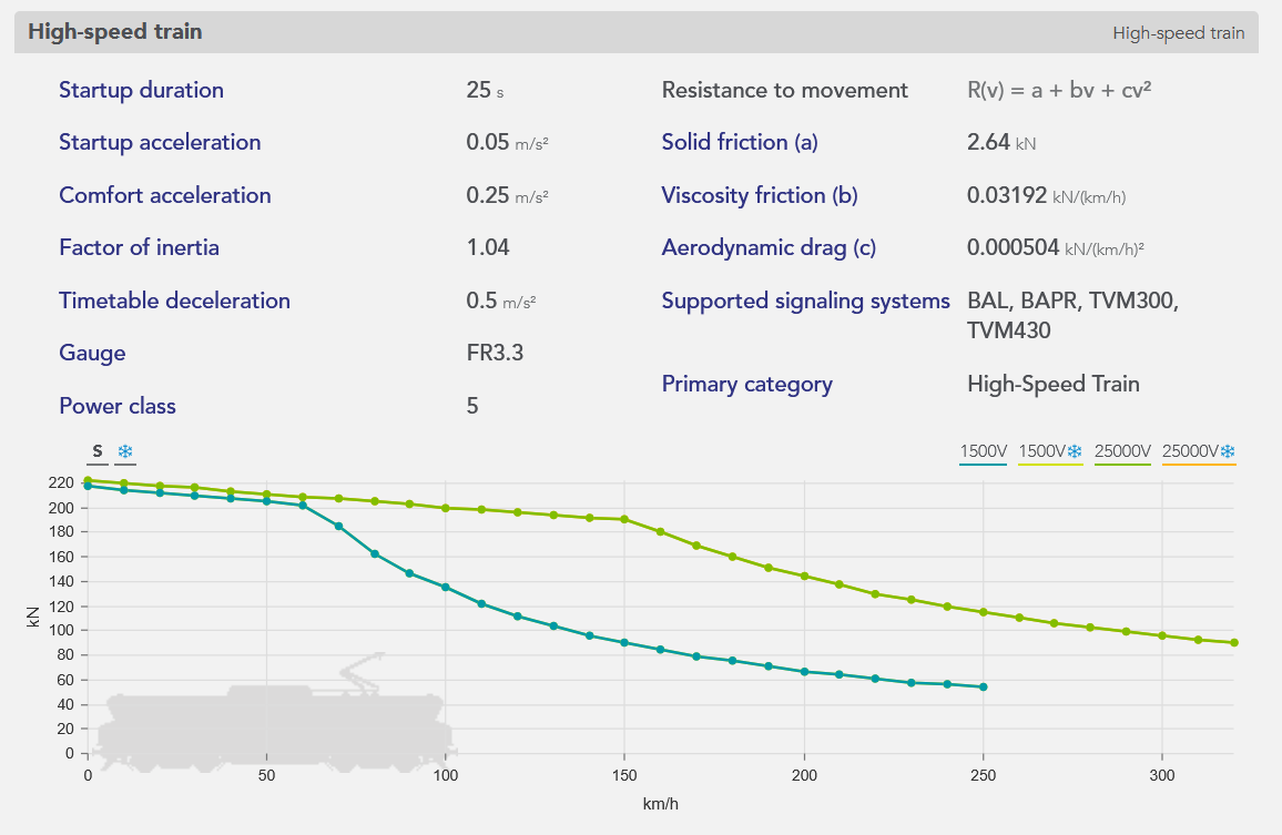
- The rolling stock: The characteristics of which needed to perform the simulation are shown below.

The orange curve, called the effort-speed curve, represents the maximum motor effort as a function of the speed of travel.
The length, mass, and maximum speed of the train are shown at the bottom of the box.
The departure time is then used to calculate the times of passage at the various points of interest (including stations).
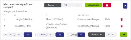
Allowances: Time added to the train’s journey to relax its running (see page on allowances).
- The time step for the calculation of numerical integration.
2 - The results
The results of a running time calculation can be represented in different forms:
- The space/time graph (GET): represents the path of trains in space and time, in the form of generally diagonal lines whose slope is the speed. Stops are shown as horizontal plates.
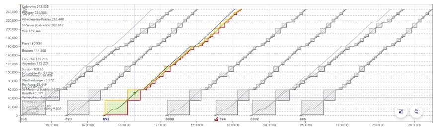
Example of a GET with several trains spaced about 30 minutes apart.
The x axis is the time of the train, the y axis is the position of the train in [m].
The blue line represents the most tense running calculation for the train, the green line represents a relaxed, so-called “economic” running calculation.
The solid rectangles surrounding the paths represent the portions of the track successively reserved for the train to pass (called blocks).
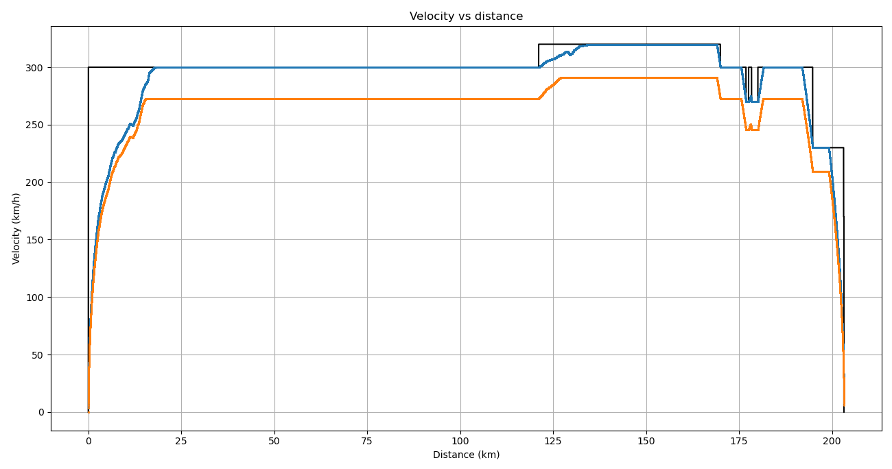
- The space/speed graph (SSG): represents the journey of a single train, this time in terms of speed. Stops are therefore shown as a drop in the curve to zero, followed by a re-acceleration.
The x axis is the train position in [m], the y axis is the train speed in [km/h].
The purple line represents the maximum permitted speed.
The blue line represents the speed in the case of the most stretched running calculation.
The green line represents the speed in the case of the “economic” travel calculation.
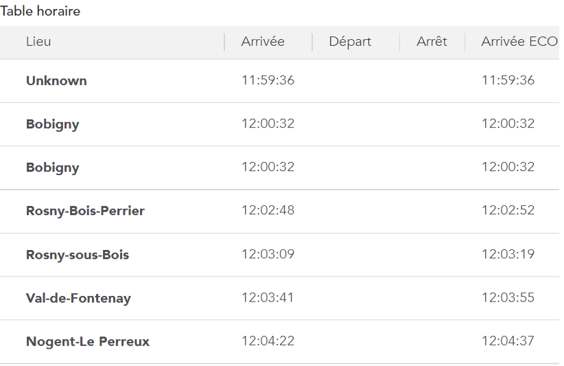
- The timetable for the passage of the train at the various points of interest.
1.3.1 - Physical modeling
Physical modelling plays an important role in the OSRD core calculation. It allows us to simulate train traffic, and it must be as realistic as possible train traffic, and it must be as realistic as possible.
Force review
To calculate the displacement of the train over time, we must first calculate its speed at each instant. A simple way to obtain this speed is to calculate the acceleration. Thanks to the fundamental principle of dynamics, the acceleration of the train at each instant is directly dependent on the different forces applied to it: $$ \sum \vec{F}=m\vec{a} $$
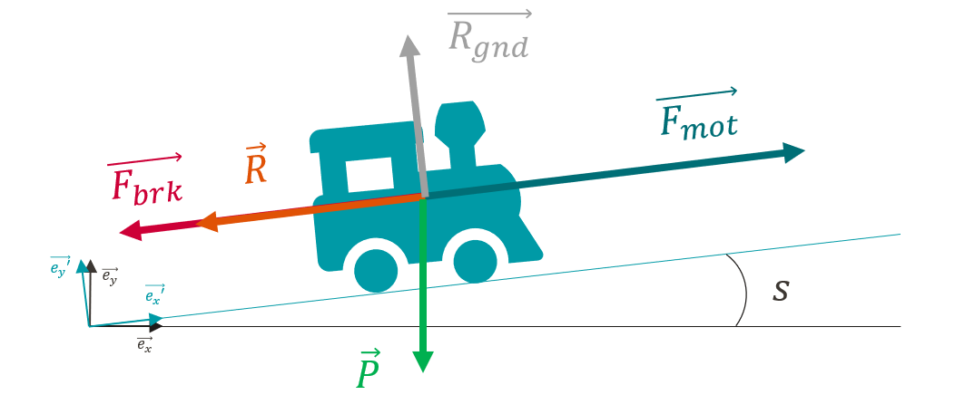
Traction: The value of the traction force \(F_{mot}\) depends on several factors:
- the rolling stock
- the speed of the train, \(v^{\prime}x\) according to the effort-speed curve below:
$$ {\vec{F_{mot}}(v_{x^{\prime}}, x^{\prime})=F_{mot}(v_{x^{\prime}}, x^{\prime})\vec{e_x^{\prime}}} $$

The x axis represents the speed of the train in [km/h], the y axis the value of the traction force in [kN].
- the action of the driver, who accelerates more or less strongly depending on where he is on his journey
- Braking : The value of the braking force \(F_{brk}\) also depends on the rolling stock and the driver’s action but has a constant value for a given rolling stock. In the current state of modelling, braking is either zero or at its maximum value.
$$ \vec{F_{brk}}(x^{\prime})=-F_{brk}(x^{\prime}){\vec{e_{x^{\prime}}}} $$
A second approach to modelling braking is the so-called hourly approach, as it is used for hourly production at SNCF. In this case, the deceleration is fixed and the braking no longer depends on the different forces applied to the train. Typical deceleration values range from 0.4 to 0.7m/s².
- Forward resistance: To model the forward resistance of the train, the Davis formula is used, which takes into account all the friction and aerodynamic resistance of the air. The value of the drag depends on the speed \(v^{\prime}_x\). The coefficients \(A\), \(B\), et \(C\) depend on the rolling stock.
$$ {\vec{R}(v_{x^{\prime}})}=-(A+Bv_{x^{\prime}}+{Cv_{x^{\prime}}}^2){\vec{e_{x^{\prime}}}} $$
- Weight (slopes + turns) : The weight force given by the product between the mass \(m\) of the train and the gravitational constant \(g\) is projected on the axes \(\vec{e_x}^{\prime}\) and \(\vec{e_y}^{\prime}\).For projection, we use the angle \(i(x^{\prime})\), which is calculated from the slope angle \(s(x^{\prime})\) corrected by a factor that takes into account the effect of the turning radius \(r(x^{\prime})\).
$$ \vec{P(x^{\prime})}=-mg\vec{e_y}(x^{\prime})= -mg\Big[sin\big(i(x^{\prime})\big){\vec{e_{x^{\prime}}}(x^{\prime})}+cos\big(i(x^{\prime})\big){\vec{e_{{\prime}}}(x^{\prime})}\Big] $$
$$ i(x^{\prime})= s(x^{\prime})+\frac{800m}{r(x^{\prime})} $$
- Ground Reaction : The ground reaction force simply compensates for the vertical component of the weight, but has no impact on the dynamics of the train as it has no component along the axis \({\vec{e_x}^{\prime}}\).
$$ \vec{R_{gnd}}=R_{gnd}{\vec{e_{y^{\prime}}}} $$
Forces balance
The equation of the fundamental principle of dynamics projected onto the axis \({\vec{e_x}^{\prime}}\) (in the train frame of reference) gives the following scalar equation:
$$ a_{x^{\prime}}(t) = \frac{1}{m}\Big [F_{mot}(v_{x^{\prime}}, x^{\prime})-F_{brk}(x^{\prime})-(A+Bv_{x^{\prime}}+{Cv_{x^{\prime}}}^2)-mgsin(i(x^{\prime}))\Big] $$
This is then simplified by considering that despite the gradient the train moves on a plane and by amalgamating \(\vec{e_x}\) and \(\vec{e_x}^{\prime}\). The gradient still has an impact on the force balance, but it is assumed that the train is only moving horizontally, which gives the following simplified equation:
$$ a_{x}(t) = \frac{1}{m}\Big[F_{mot}(v_{x}, x)-F_{brk}(x)-(A+Bv_{x}+{Cv_{x}}^2)-mgsin(i(x))\Big] $$
Resolution
The driving force and the braking force depend on the driver’s action (he decides to accelerate or brake more or less strongly depending on the situation). This dependence is reflected in the dependence of these two forces on the position of the train. The weight component is also dependent on the position of the train, as it comes directly from the slopes and bends below the train.
In addition, the driving force depends on the speed of the train (according to the speed effort curve) as does the resistance to forward motion. resistance.
These different dependencies make it impossible to solve this equation analytically, and the acceleration of the train at each moment must be calculated by numerical integration.
1.3.2 - Numerical integration
Introduction
Since physical modelling has shown that the acceleration of the train is influenced by various factors that vary along the route (gradient, curvature, engine traction force, etc.), the calculation must be carried out using a numerical integration method. The path is then separated into sufficiently short steps to consider all these factors as constant, which allows this time to use the equation of motion to calculate the displacement and speed of the train.
Euler’s method of numerical integration is the simplest way of doing this, but it has a number of drawbacks. This article explains the Euler method, why it is not suitable for OSRD purposes and which integration method should be used instead.
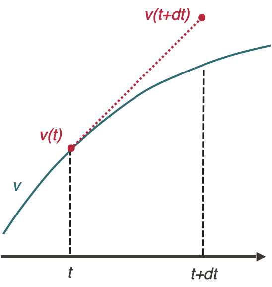
Euler’s method
The Euler method applied to the integration of the equation of motion of a train is:
$$v(t+dt) = a(v(t), x(t))dt + v(t)$$
$$x(t+dt) = \frac{1}{2}a(v(t), x(t))dt^2 + v(t)dt + x(t)$$
Advantages of Euler’s method
The advantages of the Euler method are that it is very simple to implement and has a rather fast calculation for a given time step, compared to other numerical integration methods (see appendix)
Disadvantages of the Euler’s method
The Euler integration method presents a number of problems for OSRD:
- It is relatively imprecise, and therefore requires a small time step, which generates a lot of data.
- With time integration, only the conditions at the starting point of the integration step (gradient, infrastructure parameters, etc.) are known, as one cannot predict precisely where it will end.
- We cannot anticipate future changes in the directive: the train only reacts by comparing its current state with its set point at the same time. To illustrate, it is as if the driver is unable to see ahead, whereas in reality he anticipates according to the signals, slopes and bends he sees ahead.
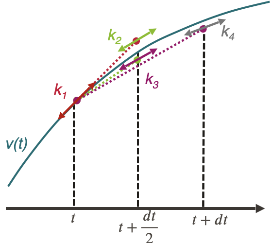
Runge-Kutta’s 4 method
The Runge-Kutta 4 method applied to the integration of the equation of motion of a train is:
$$v(t+dt) = v(t) + \frac{1}{6}(k_1 + 2k_2 + 2k_3 + k_4)dt$$
With:
$$k_1 = a(v(t), x(t))$$
$$k_2 = a\Big(v(t+k_1\frac{dt}{2}), x(t) + v(t)\frac{dt}{2} + k_1\frac{dt^2}{8}\Big)$$
$$k_3 = a\Big(v(t+k_2\frac{dt}{2}), x(t) + v(t)\frac{dt}{2} + k_2\frac{dt^2}{8}\Big)$$
$$k_4 = a\Big(v(t+k_3dt), x(t) + v(t)dt + k_3\frac{dt^2}{2}\Big)$$
Advantages of Runge Kutta’s 4 method
Runge Kutta’s method of integration 4 addresses the various problems raised by Euler’s method:
- It allows the anticipation of directive changes within a calculation step, thus representing more accurately the reality of driving a train.
- It is more accurate for the same calculation time (see appendix), allowing for larger integration steps and therefore fewer data points.
Disadvantages of Runge Kutta’s 4 method
The only notable drawback of the Runge Kutta 4 method encountered so far is its difficulty of implementation.
The choice of integration method for OSRD
Study of accuracy and speed of calculation
Different integration methods could have replaced the basic Euler integration in the OSRD algorithm. In order to decide which method would be most suitable, a study of the accuracy and computational speed of different methods was carried out. This study compared the following methods:
- Euler
- Euler-Cauchy
- Runge-Kutta 4
- Adams 2
- Adams 3
All explanations of these methods can be found (in French) in this document, and the python code used for the simulation is here.
The simulation calculates the position and speed of a high-speed train accelerating on a flat straight line.
Equivalent time step simulations
A reference curve was simulated using the Euler method with a time step of 0.1s, then the same path was simulated using the other methods with a time step of 1s. It is then possible to simply compare each curve to the reference curve, by calculating the absolute value of the difference at each calculated point. The resulting absolute error of the train’s position over its distance travelled is as follows:
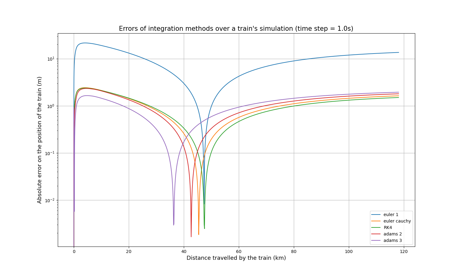
It is immediately apparent that the Euler method is less accurate than the other four by about an order of magnitude. Each curve has a peak where the accuracy is extremely high (extremely low error), which is explained by the fact that all curves start slightly above the reference curve, cross it at one point and end slightly below it, or vice versa.
As accuracy is not the only important indicator, the calculation time of each method was measured. This is what we get for the same input parameters:
| Integration method | Calculation time (s) |
|---|---|
| Euler | 1.86 |
| Euler-Cauchy | 3.80 |
| Runge-Kutta 4 | 7.01 |
| Adams 2 | 3.43 |
| Adams 3 | 5.27 |
Thus, Euler-Cauchy and Adams 2 are about twice as slow as Euler, Adams 3 is about three times as slow, and RK4 is about four times as slow. These results have been verified on much longer simulations, and the different ratios are maintained.
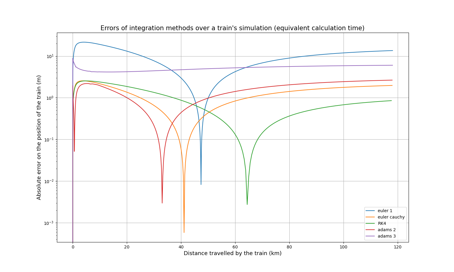
Simulation with equivalent calculation time
As the computation times of all methods depend linearly on the time step, it is relatively simple to compare the accuracy for approximately the same computation time. Multiplying the time step of Euler-Cauchy and Adams 2 by 2, the time step of Adams 3 by 3, and the time step of RK4 by 4, here are the resulting absolute error curves:
And here are the calculation times:
| Integration method | Calculation time (s) |
|---|---|
| Euler | 1.75 |
| Euler-Cauchy | 2.10 |
| Runge-Kutta 4 | 1.95 |
| Adams 2 | 1.91 |
| Adams 3 | 1.99 |
After some time, RK4 tends to be the most accurate method, slightly more accurate than Euler-Cauchy, and still much more accurate than the Euler method.
Conclusions of the study
The study of accuracy and computational speed presented above shows that RK4 and Euler-Cauchy would be good candidates to replace the Euler algorithm in OSRD: both are fast, accurate, and could replace the Euler method without requiring large implementation changes because they only compute within the current time step. It was decided that OSRD would use the Runge-Kutta 4 method because it is slightly more accurate than Euler-Cauchy and it is a well-known method for this type of calculation, so it is very suitable for an open-source simulator.
1.3.3 - Envelopes system
The envelope system is an interface created specifically for the OSRD gait calculation. It allows you to manipulate different space/velocity curves, to slice them, to end them, to interpolate specific points, and to address many other needs necessary for the gait calculation.
A specific interface in the OSRD Core service
The envelope system is part of the core service of OSRD (see software architecture).
Its main components are :
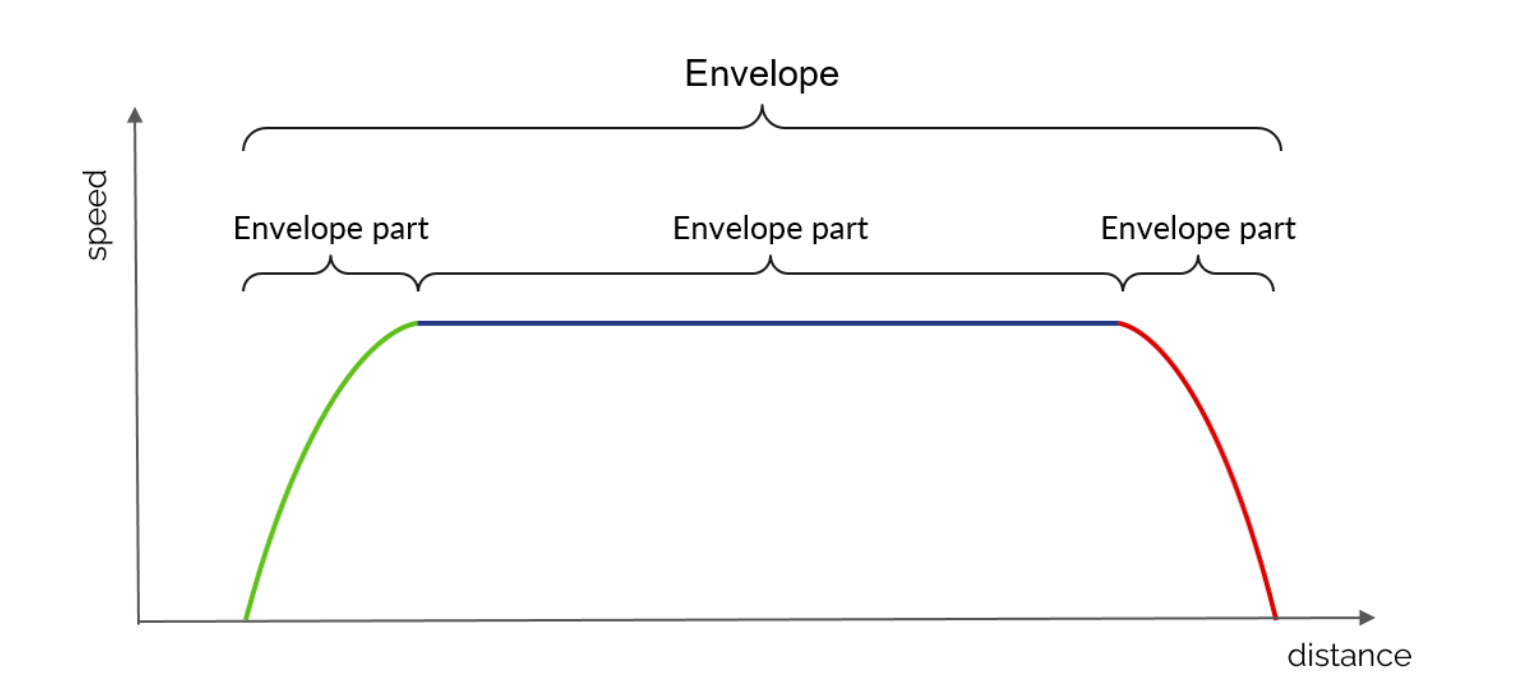
1 - EnvelopePart: space/speed curve, defined as a sequence of points and having metadata indicating for example if it is an acceleration curve, a braking curve, a speed hold curve, etc.
2 - Envelope: a list of end-to-end EnvelopeParts on which it is possible to perform certain operations:
- check for continuity in space (mandatory) and speed (optional)
- look for the minimum and/or maximum speed of the envelope
- cut a part of the envelope between two points in space
- perform a velocity interpolation at a certain position
- calculate the elapsed time between two positions in the envelope
3 - Overlays : system for adding more constrained (i.e. lower speed) EnvelopeParts to an existing envelope.
Given envelopes vs. calculated envelopes
During the simulation, the train is supposed to follow certain speed instructions. These are modelled in OSRD by envelopes in the form of space/speed curves. Two types can be distinguished:
- Envelopes from infrastructure and rolling stock data, such as maximum line speed and maximum train speed. Being input data for our calculation, they do not correspond to curves with a physical meaning, as they are not derived from the results of a real integration of the physical equations of motion.
- The envelopes result from real integration of the physical equations of motion. They correspond to a curve that is physically tenable by the train and also contain time information.
A simple example to illustrate this difference: if we simulate a TER journey on a mountain line, one of the input data will be a maximum speed envelope of 160km/h, corresponding to the maximum speed of our TER. However, this envelope does not correspond to a physical reality, as it is possible that on certain sections the gradient is too steep for the train to be able to maintain this maximum speed of 160km/h. The calculated envelope will therefore show in this example a speed drop in the steepest areas, where the envelope given was perfectly flat.
Simulation of several trains
In the case of the simulation of many trains, the signalling system must ensure safety. The effect of signalling on the running calculation of a train is reproduced by superimposing dynamic envelopes on the static envelope. A new dynamic envelope is introduced for example when a signal closes. The train follows the static economic envelope superimposed on the dynamic envelopes, if any. In this simulation mode, a time check is performed against a theoretical time from the time information of the static economic envelope. If the train is late with respect to the scheduled time, it stops following the economic envelope and tries to go faster. Its space/speed curve will therefore be limited by the maximum effort envelope.
1.3.4 - Pipeline
The walk calculation in OSRD is a 4-step process, each using the envelopes system:
- Construction of the most restrictive speed profile
- Addition of the different braking curves
- Adding the different acceleration curves and checking the constant speed curves
- Application of allowance(s)
Calculation of the Most Restricted Speed Profile (MRSP)
A first envelope is calculated at the beginning of the simulation by grouping all static velocity limits:
- maximum line speed
- maximum speed of rolling stock
- temporary speed limits (e.g. in case of works on a line)
- speed limits by train category
- speed limits according to train load
- speed limits corresponding to signposts
The length of the train is also taken into account to ensure that the train does not accelerate until its tail leaves the slowest speed zone. An offset is then applied to the red dashed curve. The resulting envelope (black curve) is called the Most Restricted Speed Profile (MRSP). It is on this envelope that the following steps will be calculated.
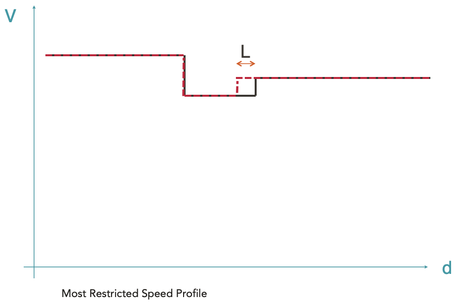
The red dotted line represents the maximum permitted speed depending on the position. The black line represents the MRSP where the train length has been taken into account.
It should be noted that the different envelopeParts composing the MRSP are input data, so they do not correspond to curves with a physical reality.
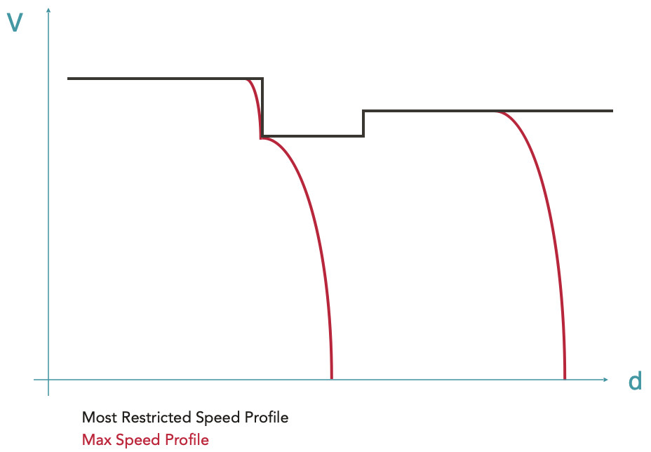
Calculation of the Max Speed Profile
Starting from the MRSP, all braking curves are calculated using the overlay system (see here for more details on overlays), i.e. by creating envelopeParts which will be more restrictive than the MRSP. The resulting curve is called Max Speed Profile. This is the maximum speed envelope of the train, taking into account its braking capabilities.
Since braking curves have an imposed end point and the braking equation has no analytical solution, it is impossible to predict their starting point. The braking curves are therefore calculated backwards from their target point, i.e. the point in space where a certain speed limit is imposed (finite target speed) or the stopping point (zero target speed).
For historical reasons in hourly production, braking curves are calculated at SNCF with a fixed deceleration, the so-called hourly deceleration (typically ~0.5m/s²) without taking into account the other forces. This method has therefore also been implemented in OSRD, allowing the calculation of braking in two different ways: with this hourly rate or with a braking force that is simply added to the other forces.
Calculation of the Max Effort Profile
For each point corresponding to an increase in speed in the MRSP or at the end of a stop braking curve, an acceleration curve is calculated. The acceleration curves are calculated taking into account all active forces (traction force, driving resistance, weight) and therefore have a physical meaning.
For envelopeParts whose physical meaning has not yet been verified (which at this stage are the constant speed running phases, always coming from the MRSP), a new integration of the equations of motion is performed. This last calculation is necessary to take into account possible speed stalls in case the train is physically unable to hold its speed, typically in the presence of steep ramps (see this example).
The envelope that results from the addition of the acceleration curves and the verification of the speed plates is called the Max Effort Profile.
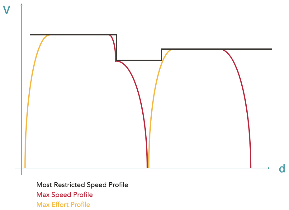
At this stage, the resulting envelope is continuous and has a physical meaning from start to finish. The train accelerates to the maximum, runs as fast as possible according to the different speed limits and driving capabilities, and brakes to the maximum. The resulting travel calculation is called the basic running time. It corresponds to the fastest possible route for the given rolling stock on the given route.
Application of allowance(s)
After the calculation of the basic run (corresponding to the Max Effort Profile in OSRD), it is possible to apply allowances. Allowances are additions of extra time to the train’s journey. They are used to allow the train to catch up if necessary or for other operational purposes (more details on allowances here).
A new Allowances envelope is therefore calculated using overlays to distribute the allowance requested by the user over the maximum effort envelope calculated previously.
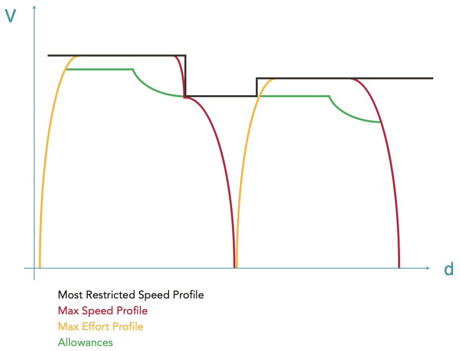
In the OSRD running calculation it is possible to distribute the allowances in a linear way, by lowering all speeds by a certain factor, or in an economic way, i.e. by minimising the energy consumption during the train run.
1.3.5 - Allowances
The purpose of allowances
As explained in the calculation of the Max Effort Profile, the basic running time represents the most stretched run normally achievable, i.e. the fastest possible run of the given equipment on the given route. The train accelerates to the maximum, travels as fast as possible according to the different speed limits and driving capabilities, and brakes to the maximum.
This basic run has a major disadvantage: if a train leaves 10 minutes late, it will arrive at best 10 minutes late, because by definition it is impossible for it to run faster than the basic run. Therefore, trains are scheduled with one or more allowances added. The allowances are a relaxation of the train’s route, an addition of time to the scheduled timetable, which inevitably results in a lowering of running speeds.
A train running in basic gear is unable to catch up!
Allowances types
There are two types of allowances:
- The regularity allowance: this is the additional time added to the basic running time to take account of the inaccuracy of speed measurement, to compensate for the consequences of external incidents that disrupt the theoretical run of trains, and to maintain the regularity of the traffic. The regularity allowance applies to the whole route, although its value may change at certain intervals.
- The construction allowance: this is the time added/removed on a specific interval, in addition to the regularity allowance, but this time for operational reasons (dodging another train, clearing a track more quickly, etc.)
A basic running time with an added allowance of regularity gives what is known as a standard walk.
Allowance distribution
Since the addition of allowance results in lower speeds along the route, there are a number of possible routes. Indeed, there are an infinite number of solutions that result in the same journey time.
As a simple example, in order to reduce the running time of a train by 10% of its journey time, it is possible to extend any stop by the time equivalent to this 10%, just as it is possible to run at 1/1.1 = 90.9% of the train’s capacity over the entire route, or to run slower, but only at high speeds…
There are currently two algorithms for margin distribution in OSRD: linear and economic.
Linear distribution
Linear allowance distribution is simply lowering the speeds by the same factor over the area where the user applies the allowance. Here is an example of its application:
The advantage of this distribution is that the allowance is spread evenly over the entire journey. A train that is late on 30% of its journey will have 70% of its allowance for the remaining 70% of its journey.
Economic distribution
The economic distribution of the allowance, presented in detail in this document (MARECO is an algorithm designed by the SNCF research department), consists of distributing the allowance in the most energy-efficient way possible. It is based on two principles:
- a maximum speed, avoiding the most energy-intensive speeds
- run-on zones, located before braking and steep gradients, where the train runs with the engine off thanks to its inertia, allowing it to consume no energy during this period
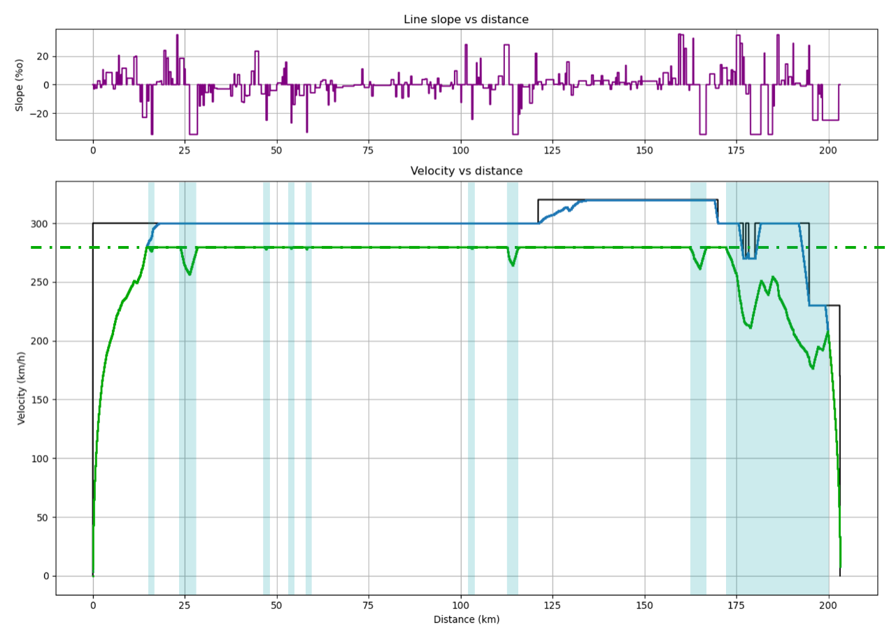
An example of economic walking. Above, the gradients/ramps encountered by the train. The areas of travel on the track are shown in blue.
1.4 - Netzgrafik-Editor
Open-source software developed by SBB CFF FFS and its integration in OSRD
Netzgrafik-Editor (NGE) is an open-source software that enables the creation, modification, and analysis of regular-interval timetable, at a macroscopic level of detail, developed by Swiss Federal Railways (SBB CFF FFS). See front-end and back-end repositories.
OSRD and NGE are are semantically different: the former uses a microscopic level of detail, based on a well-defined infrastructure, depicting a timetable composed of unique train schedules, while the latter uses a macroscopic level of detail, not based on any explicit infrastructure, depicting a transportation plan made up of regular-interval based train runs. However, these differences, close enough, may be arranged to make it work together.
The compatibility between NGE and OSRD has been tested through a proof of concept, by running both pieces of software as separate services and without automated synchronization.
The idea is to give to OSRD a graphical tool to edit (create, update and delete train schedules from) a timetable from an operational study scenario, and get some insights on analytics at the same time. Using both microscopic and macroscopic levels of detail brings a second benefit: OSRD’s microscopic calculations extend the actual scope of NGE, its functionalities and information provided, such as the microscopic simulations or the conflicts detection tool.
The transversal objective of this feature is to make two open-source projects from two big railway infrastructure managers work along and cooperate with one another with the same goal: ensure a digital continuity on different time scales for railway operational studies.
1 - Integration in OSRD
OSRD has developed a standalone version of NGE, integrated into the source code, which allows NGE to work without a back-end. Thus, for external use, a build of NGE standalone is available on NPM and is published at each release. Finally, to meet OSRD-specific needs, OSRD uses a fork of NGE (whose build, NGE standalone, is also available on NPM), remaining as close as possible to the official directory.
Despite using different JavaScript frameworks (ReactJS for OSRD and Angular for NGE), this build allows OSRD to integrate NGE within an iframe. This iframe instantiates a Custom Element, which is be the communication interface between both applications and launch NGE’s build.
An alternative solution to the integration problem would have been to rewrite NGE as web-components, in order to import them into OSRD, but this solution was abandoned because of the amount of work it would represent.
NGE, in its standalone version, communicates with OSRD through the iframe using DOM element properties:
@Input: with thenetzgrafikDtoproperty, triggered when the content of the scenario is updated from OSRD.@Output: with theoperationsproperty, triggered when NGE is used.
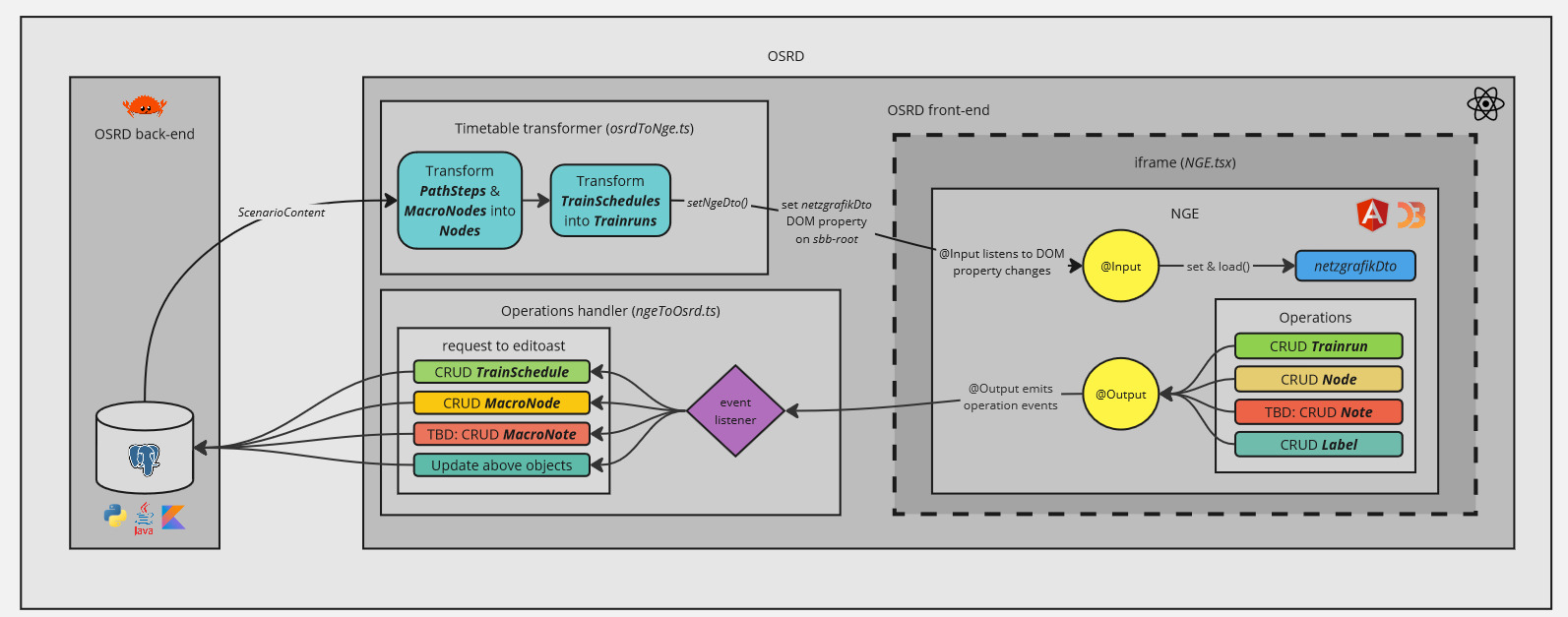
NGE is then able to obtain the OSRD timetable as soon as a change is made on the OSRD side, and OSRD is able to obtain the changes made on the NGE side.
2 - Converters
To overcome semantic differences and adapt data models, two converters are implemented:
- [OSRD -> NGE] a converter which transforms an OSRD timetable into an NGE model. The nodes are the waypoints described by the train schedules, and whose macroscopic information (position on the reticular) is stored in the database. OSRD train schedules,
TrainSchedule, then represent cadenced train lines in NGE,Trainrun. A concept of cadenced train lines, will soon be implemented to allow conceptual convergence between OSRD and NGE. - [OSRD <- NGE] an event manager, which transforms an NGE action into an update of the OSRD database.
3 - Open-source (cooperation / contribution)
To make NGE compatible with OSRD, some changes have been requested (disable back-end, create hooks on events) and directly implemented in the official repository of NGE, with the agreement and help of NGE team.
Contributions for one project to another, from both sides, are valuable and will be entertained in the future.
This feature also shows that open-source cooperation is powerful and a huge gain of time in software development.
2 - How-to Guides
Recipes for addressing key problems and use-cases
How-to guides are recipes. They guide you through the steps involved in addressing key problems and use-cases. They are more advanced than tutorials and assume some knowledge of how OSRD works.
2.1 - Contribute to OSRD
Learn about the how we work, and how you can work with us
2.1.1 - Preamble
An introduction to contributing to OSRD
First off, thanks for taking the time to contribute!
The following chapters are a set of guidelines for contributing to OSRD. These guidelines are mostly not strict rules, it’s probably fine to do things slightly differently. If you have already contributed to open source projects before, you probably won’t be surprised. If you have not, it will probably help a lot!
Communicate
Chatting with other contributors is a great way to speed things up:
- Create an issue to discuss your contribution project.
Inquire
Just like with any project, changes rely on past work. Before making changes, it is best to learn about what’s already there:
- read technical documentation
- read the existing source code related to your project
- chat with developers who last worked on areas you are interested in
2.1.2 - License and set-up
How to set up your development environment? What does our license involve?
License of code contributions
The source code of OSRD is available under the LGPLv3 license. By contributing to the codebase, you consent to the distribution of your changes under the project’s license.
LGPLv3 forbids modifying source code without sharing the changes under the same license: use other people’s work, and share yours!
This constraint does not propagate through APIs: You can use OSRD as a library, framework or API server to interface with proprietary software. Please suggest changes if you need new interfaces.
Set things up
Most OSRD developers use Linux (incl. WSL). Windows and MacOS should work too, but you may run into some issues.
Get the source code
- Install
git.1 - Open a terminal2 in the folder where the source code of OSRD will be located
- Run
git clone https://github.com/OpenRailAssociation/osrd.git
Launch the application
Docker is a tool which greatly reduces the amount of setup required to work on OSRD:
- download the latest development build:
docker compose pull - start OSRD:
docker compose up - build and start OSRD:
docker compose up --build - review a PR using CI built images:
TAG=pr-XXXXX docker compose up --no-build --pull always
To get started:
- Install
docker - Follow OSRD’s README.
2.1.3 - Contribute code
Integrate changes into OSRD
This chapter is about the process of integrating changes into the common code base. If you need help at any stage, open an issue or message us.
OSRD application is split in multiple services written in several languages. We try to follow general code best practices and follow each language specificities when required.
2.1.3.1 - General principles
Please read this first!
- Explain what you’re doing and why.
- Document new code with doc comments.
- Include clear, simple tests.
- Break work into digestible chunks.
- Take the time to pick good names.
- Avoid non well-known abbreviations.
- Control and consistency over 3rd party code reuse: Only add a dependency if it is absolutely necessary.
- Every dependency we add decreases our autonomy and consistency.
- We try to keep PRs bumping dependencies to a low number each week in each component, so grouping
dependency bumps in a batch PR is a valid option (see component’s
README.md). - Don’t reinvent every wheel: as a counter to the previous point, don’t reinvent everything at all costs.
- If there is a dependency in the ecosystem that is the “de facto” standard, we should heavily consider using it.
- More code general recommendations in main repository CONTRIBUTING.md.
- Ask for any help that you need!
Consult back-end conventions ‣
2.1.3.2 - Back-end conventions
Coding style guide and best practices for back-end
Python
Python code is used for some packages and integration testing.
- Follow the Zen of Python.
- Projects are organized with uv
- Code is linted with ruff.
- Code is formatted with ruff.
- Python tests are written using pytest.
- Typing is checked using pyright.
Rust
- As a reference for our API development we are using the Rust API guidelines. Generally, these should be followed.
- Prefer granular imports over glob imports like
diesel::*. - Tests are written with the built-in testing framework.
- Use the documentation example to know how to phrase and format your documentation.
- Use consistent comment style:
///doc comments belong above#[derive(Trait)]invocations.//comments should generally go above the line in question, rather than in-line.- Start comments with capital letters. End them with a period if they are sentence-like.
- Use comments to organize long and complex stretches of code that can’t sensibly be refactored into separate functions.
- Code is linted with clippy.
- Code is formatted with fmt.
Java
- Code is formatted with checkstyle.
2.1.3.3 - Front-end conventions
Coding style guide and best practices for front-end
We use ReactJS and all files must be written in Typescript.
The code is linted with eslint, and formatted with prettier.
Nomenclature

The applications (osrd eex, osrd stdcm, infra editor, rolling-stock editor) offer views (project management, study management, etc.) linked to modules (project, study, etc.) which contain the components.
These views are made up of components and sub-components all derived from the modules. In addition to containing the views files for the applications, they may also contain a scripts directory which offers scripts related to these views. The views determine the logic and access to the store.
Modules are collections of components attached to an object (a scenario, a rolling stock, a TrainSchedule). They contain :
- a components directory hosting all components
- an optional styles directory per module for styling components in scss
- an optional assets directory per module (which contains assets, e.g. default datasets, specific to the module)
- an optional reducers file per module
- an optional types file per module
- an optional consts file per module
An assets directory (containing images and other files).
Last but not least, a common directory offering :
- a utils directory for utility functions common to the entire project
- a types file for types common to the entire project
- a consts file for constants common to the entire project
Implementation principles
Naming
The following conventions are generally used in the code:
- components and types are in PascalCase
- variables are in camelCase
- translation keys are also in camelCase
- constants are in SCREAMING_SNAKE_CASE (except in special cases)
- CSS classes are in kebab-case
Styles & SCSS
WARNING: in CSS/React, the scope of a class does not depend on where the file is imported, but is valid for the entire application. If you import an
scssfile in the depths of a component (which we strongly advise against), its classes will be available to the whole application and may therefore cause side effects.
It is therefore highly recommended to be able to easily follow the tree structure of applications, views, modules and components also within the SCSS code, and in particular to nest class names to avoid edge effects.
Some additional conventions:
- All sizes are expressed in px, except for fonts which are expressed in rem.
- We use the classnames library to conditionally apply classes: each class is separated into a string, and Boolean or other operations are performed in an object that will return—or not—the property name as the class name to be used in CSS.
Store/Redux
The store allows you to store data that will be accessible anywhere in the application. It is divided into slices, which correspond to our applications.
However, we must be careful that our store does not become a catch-all. Adding new properties to the store must be justified by the fact that the data in question is “high-level” and will need to be accessible from locations far from each other, and that a simple state or context variable is not appropriate for storing this information.
For more details about redux, please refer to the official documentation.
Redux ToolKit (RTK)
We use Redux ToolKit to make our calls to the backend.
RTK allows you to make API calls and cache responses. For more details, please refer to the official documentation.
The backend endpoints and types are generated directly from the editoast open API and stored in generatedOsrdApi (using the npm run generate-types command). This generated file is then enriched with other endpoints or types in osrdEditoastApi, which can be used in the application. Note that it is possible to transform mutations into queries when generating generatedOsrdApi by modifying the openapi-editoast-config file.
When an endpoint call must be skipped because a variable is not defined, RTK’s skipToken is used to avoid having to use casts.
Translation
Application translation is performed on Weblate.
Imports
It is recommended that you use the full path for each import, unless your import file is in the same directory.
ESLint is setup to automatically sort imports in four import groups, each of them separated by an empty line and sorted in alphabetical order :
- React
- External libraries
- Internal absolute path files
- Internal relative path files
Regarding type imports/exports, ESLint and Typescript are configured to automatically add type before a type import, which allows to:
- Improve the performance and analysis process of the compiler and the linter.
- Make these declarations more readable; we can clearly see what we are importing.
- Make final bundle lighter (all types disappear at compilation)
- Avoid dependency cycles (ex: the error disappears with the
typekeyword)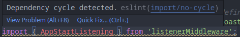

2.1.3.4 - Write code
Integrate changes into OSRD
If you are not used to Git, follow this tutorial
Create a branch
If you intend to contribute regularly, you can request access to the main repository. Otherwise, create a fork.Add changes to your branch
Before you start working, try to split your work into macroscopic steps. At the end of each stop, save your changes into a commit. Try to make commits of logical and atomic units. Try to follow style conventions (back-end and front-end).Keep your branch up-to-date
git switch <your_branch>
git fetch
git rebase origin/dev
2.1.3.5 - Commit conventions
A few tips and rules about commit messages
Commit style
The overall format for git commits is as follows:
component1, component2: imperative description of the change

Detailed or technical description of the change and what motivates it,
if it is not entirely obvious from the title.
- the commit message, just like the code, must be in English (only ASCII characters for the title)
- there can be multiple components separated by
:in case of hierarchical relationships, with,otherwise - components are lower-case, using
-,_or.if necessary - the imperative description of the change begins with a lower-case verb
- the title must not contain any link (
#is forbidden)
Ideally:
- the title should be self-explanatory: no need to read anything else to understand it
- the commit title is all lower-case
- the title is clear to a reader not familiar with the code
- the body of the commit contains a detailed description of the change
An automated check is performed to enforce as much as possible this formatting.
Counter-examples of commit titles
To be avoided entirely:
component: update ./some/file.ext: specify the update itself rather than the file, the files are technical elements welcome in the body of the commitcomponent: fix #42: specify the problem fixed in the title, links (to issue, etc.) are very welcome in commit’s bodywip: describe the work (and finish it)
Welcome to ease review, but do not merge:
fixup! previous commit: an autosquash must be run before the mergeRevert "previous commit of the same PR": both commits must be dropped before merging
The Developer Certificate of Origin (DCO)
All of OSRD’s projects use the DCO (Developer Certificate of Origin) to address legal matters. The DCO helps confirm that you have the rights to the code you contribute. For more on the history and purpose of the DCO, you can read The Developer Certificate of Origin by Roscoe A. Bartlett.
To comply with the DCO, all commits must include a Signed-off-by line.
How to sign a commit using git in a shell ?
To sign off a commit, simply add the -s flags to your git commit command,
like so:
git commit -s -m "Your commit message"
This also applies when using the git revert command.
How to do sign a commit using git in Visual Studio Code (VS Code) ?
Now, go in Files -> Preferences -> Settings, search for and activate
the Always Sign Off setting.
Finally, when you’ll commit your changes via the VS Code interface, your commits will automatically be signed-off.
2.1.3.6 - Share your changes
How to submit your code modifications for review?
The author of a pull request (PR) is responsible for its “life cycle”. He is responsible for contacting the various parties involved, following the review, responding to comments and correcting the code following review (you could also check dedicated page about code review).
Open a pull request
Once your changes are ready, you have to request integration with thedevbranch.If possible:
- Make PR of logical and atomic units too (avoid mixing refactoring, new features and bug fix at the same time).
- Add a description to PRs to explain what they do and why.
- Help the reviewer by following advice given in mtlynch article.
- Add tags
area:<affected_area>to show which part of the application have been impacted. It can be done through the web interface.
Take feedback into account
Once your PR is open, other contributors can review your changes:- Any user can review your changes.
- Your code has to be approved by a contributor familiar with the code.
- All users are expected to take comments into account.
- Comments tend to be written in an open and direct manner. The intent is to efficiently collaborate towards a solution we all agree on.
- Once all discussions are resolved, a maintainer integrates the change.
The best case is to avoid large PR and split it in multiple PR1:
- ease the reviewing process and might accelerate it (easier to find an hour to review than half a day)
- is more agile, you will get feedback on the early iteration before proposing the next series of modifications,
- keep the git history cleaner (in case of a
git bisectlooking for a regression for example).In the case where you cannot avoid a large PR, don’t hesitate to ask several reviewers to organize themselves, or even to carry out the review together, reviewers and author.
For large PRs that are bound to evolve over time, keeping corrections during review in separate commits helps reviewers. In the case of multiple reviews by the same person, this can save full re-review (ask for help if necessary):
- Add fixup, amend, squash or reword commits using the git commit documentation.
- Automatically merge corrections into the original commits of your PR and check the result, using
git rebase -i --autosquash origin/dev(just before the merge and once review process is complete).- Push your changes with
git push --force-with-leasebecause you are not just pushing new commits, you are pushing changes to existing commits.
- If you believe somebody forgot to review / merge your change, please speak out, multiple times if needs be.
Review cycle
A code review is an iterative process. For a smooth review, it is imperative to correctly configure your github notifications.
It is advisable to configure OSRD repositories as “Participating and @mentions”. This allows you to be notified of activities only on issues and PRs in which you participate.
Maintainers are automatically notified by the
CODEOWNERSsystem. The author of a PR is responsible for advancing their PR through the review process and manually requesting maintainer feedback if necessary.
sequenceDiagram
  actor A as PR author
  actor R as Reviewer/Maintainer

  A->>R: Asks for a review, notifying some people
  R->>A: Answers yes or no

  loop Loop between author and reviewer
    R-->>A: Comments, asks for changes
    A-->>R: Answers to comments or requested changes
    A-->>R: Makes necessary changes in dedicated "fixups"
    R-->>A: Reviews, tests changes, and comments again
    R-->>A: Resolves requested changes/conversations if ok
  end

  A->>R: Rebase and apply fixups
  R->>A: Checks commits history
  R->>A: Approves the PR
  Note right of A: Add to the merge queue
Finally continue towards tests ‣
if you are not convinced, look for “Stacked Diff” on the web for more literature on the topic, like Stacked Diffs vs. Trunk Based Development ↩︎
2.1.3.7 - Tests
Recommendations for testing purpose
Back-end
- Integration tests are written with pytest in the
/testsfolder. - Each route described in the
openapi.yamlfiles must have an integration test. - The test must check both the format and content of valid and invalid responses.
Front-end
The functional writing of the tests is carried out with the Product Owners, and the developers choose a technical implementation that precisely meets the needs expressed and fits in with the recommendations presented here.
We use Playwright to write end-to-end tests, and vitest to write unit tests.
The browsers tested are currently Firefox and Chromium.
Basic principles
- Tests must be short (1min max) and go straight to the point.
- Arbitrary timeouts are outlawed; a test must systematically wait for a specific event. It is possible to use polling (retry an action - a click for example - after a certain time) proposed in the Playwright’s API.
- All tests must be parallelizable.
- Tests must not point to or wait for text elements from the translation, prefer the DOM tree structure or place specific
id. - We’re not testing the data, but the application and its functionality. Data-specific tests should be developed in parallel.
Data
The data tested must be public data.
The data required (infrastructure and rolling stock) for the tests are offered in the application’s json files, injected at the start of each test and deleted at the end, regardless of its result or how it is stopped, including with CTRL+C.
This is done by API calls in typescript before launching the actual test.
The data tested is the same, both locally and via continuous integration.
End-to-End (E2E) Test Development Process
E2E tests are implemented iteratively and delivered alongside feature developments. Note that:
- E2E tests should only be developed for the application’s critical user journeys.
- This workflow helps prevent immediate regressions after a feature release, enhances the entire team’s proficiency in E2E testing, and avoids excessively long PRs that would introduce entire E2E test suites at once.
- It is acceptable for E2E tests to be partial during development, even if their implementation increases ticket size and development time.
- Some parts of the tests will need to be mocked while the feature is still under development. However, by the end of development, the E2E test must be complete, and all mocked data should be removed. The final modifications to eliminate mocking should be minimal (typically limited to updating expected values).
- When adding a new feature, it is preferable to separate the implementation of the new feature and the tests into individual commits, to facilitate review.
- Test cases and user journeys should be defined in advance, during ticket refinement, before the PIP. They may be proposed by a QA or a Product Owner (PO) and must be validated by a QA, the relevant PO, and frontend developers.
- If an E2E test affects the E2E testing configuration, project architecture (e.g., snapshotting), or poses a risk of slowing down the CI, a refinement workshop must be organized to consult the team responsible for project architecture and CI, particularly the DevOps team.
Atomicity of a test
Each test must be atomic: it is self-sufficient and cannot be divided.
A test will target a single feature or component, provided it is not too large. A test will not test an entire module or application; it will necessarily be a set of tests, in order to preserve test atomicity.
If a test needs elements to be created or added, these operations must be carried out by API calls in typescript upstream of the test, as is done for adding data. These elements must be deleted at the end of the test, regardless of the result or how it is stopped, including by CTRL+C.
This allows tests to be parallelized.
However, in certain cases where it is relevant, a test may contain several clearly explained and justified test subdivisions (several test() in a single describe()).
Example of a test
The requirement: “We want to test the addition of a train to a timetable”.
- add the test infrastructure and rolling stock to the database by API calls.
- create project, study and scenario with choice of test infrastructure by API calls.
- start the test, clicking on “add one or more trains” until the presence of the trains in the timetable is verified
- the test passes, fails or is stopped, the project, study and scenario are deleted, along with the test rolling stock and infrastructure by API calls.
NB: the test will not test all the possibilities offered by the addition of trains; this should be a specific test which would test the response of the interface for all scenarios without adding trains.
2.1.4 - Review process
How to give useful feedback
The reviewer/maintainer undertakes to carry out the review quickly, and is also responsible for closing request changes, check commit history and quickly merge the pull request if allowed.
We propose you a few tips and recommendations that we think are relevant to a human, relevant and rewarding code review for all contributors:
- How to Make Your Code Reviewer Fall in Love with You? by Michael Lynch.
- If you prefer audio, the FOSDEM presentation of Alya Abbott is also a good take on the topic
- How to Do Code Reviews Like a Human? by Michael Lynch.
Review cycle
A code review is an iterative process. For a smooth review, it is imperative to correctly configure your github notifications.
It is advisable to configure OSRD repositories as “Participating and @mentions”. This allows you to be notified of activities only on issues and PRs in which you participate.
Maintainers are automatically notified by the
CODEOWNERSsystem. The author of a PR is responsible for advancing their PR through the review process and manually requesting maintainer feedback if necessary.
sequenceDiagram
  actor A as PR author
  actor R as Reviewer/Maintainer

  A->>R: Asks for a review, notifying some people
  R->>A: Answers yes or no

  loop Loop between author and reviewer
    R-->>A: Comments, asks for changes
    A-->>R: Answers to comments or requested changes
    A-->>R: Makes necessary changes in dedicated "fixups"
    R-->>A: Reviews, tests changes, and comments again
    R-->>A: Resolves requested changes/conversations if ok
  end

  A->>R: Rebase and apply fixups
  R->>A: Checks commits history
  R->>A: Approves the PR
  Note right of A: Add to the merge queue
The code review pyramid

Script for testing a PR
When reviewing a PR, it is useful to test the changes by starting an instance of the OSRD app based on the PR branch.
A script is available to spin up a separate and dedicated app instance using the PR number. The script uses the Docker images already built by the CI and launches the app, running in isolation. This allows you to run both instances simultaneously without conflicts (ideal for comparing changes, for example).
Additionally, you can specify a database backup, which the script will load directly into the app.
The app will be launched on the 4001 port. You can access it at: http://localhost:4001/
Available Commands:
./scripts/pr-tests-compose.sh 8914 up: Downloads the CI-generated images for PR #8914 and launches the application../scripts/pr-tests-compose.sh 8914 up-and-load-backup ./path_to_backup: Downloads the images for PR #8914, restores data from the provided backup, and starts the application../scripts/pr-tests-compose.sh down: Shuts down the test application instance for PR #8914../scripts/pr-tests-compose.sh down-and-clean: Shuts down the test instance and cleans all the instance’s docker volumes (PG data, Valkey cache, RabbitMQ) to prevent any side-effects.
Accessing Services:
Apart from the frontend server, all localhost services are available on localhost, with a minor port adjustment (to avoid conflicts with the dev environment): for a list of common ports, have a look at the dedicated docker-compose file.
2.1.5 - Report issues
Report a bug or suggest an enhancement
Please report anything you deem significant!
Our bug tracking platform is github, so you have to register to report bugs.
Follow this link and pick whatever template fits the best.
Bugs
- Bug must have a correct description and the bug’s issue template must be filled carefully.
- Bug must be tagged with (for team members):
kind:bug- one or several
area:<affected_area>if possible, if the affected area is not known leave it blank it will be added later by another team member. - one
severity:<bug_severity>if possible, if severity is not known leave it blank it will be added later by another team member.severity:minor: User can still use the feature.severity:major: User sometimes can’t use the feature.severity:critical: User can’t use the feature.
- OSRD team members can change issues’ tags (severity, area, kind, …). You may leave a comment to explain changes.
- If you are working on a bug or plan to work on a bug, assign yourself to the bug.
- PRs solving bugs should add a regression tests to ensure that bug will not be back in the future.
2.1.6 - Install docker
Regardless of your operating system, docker requires linux to operate. When used on a different operating system, docker relies on virtual machines to build and run images.
There are two main types of docker installations:
- docker engine is the usual docker command line application
- docker desktop is a GUI app that also manages virtualization
Here’s what we suggest:
- If you’re on linux, install docker engine using your package manager
- If you’re on MacOS / Windows, install docker desktop if you are allowed to
- If you’re on windows and want to get docker running within WSL, or can’t use docker desktop, follow the docker on WSL tutorial
- If you’re on MacOS and can’t use docker desktop, follow the MacOS colima tutorial
Docker on WSL
This install option is very useful, as it allows having a perfectly normal linux install of docker engine inside WSL, which can still be reached from windows.
- Install WSL (If you had an old version of WSL, run
wsl --upgrade) - Get an operating system image from the microsoft store (for example, debian or ubuntu)
- Enable systemd support within the WSL VM
- Follow the regular linux install tutorial for docker
- If you have docker desktop installed, you can configure it to use WSL
MacOS colima
This procedure allows installing docker without relying on docker desktop. It uses colima for virtualizing linux.
- Install homebrew
brew install docker docker-compose colima- Install the compose plugin:
mkdir -p ~/.docker/cli-plugins && ln -sfn $(brew --prefix)/opt/docker-compose/bin/docker-compose ~/.docker/cli-plugins/docker-compose - Configure colima:
- for apple silicon (M1/M2) macbooks:
colima start --cpu 2 --memory 6 --arch aarch64 --vm-type=vz --vz-rosetta --mount-type=virtiofs - for small infrastructures:
colima start --cpu 2 --memory 4 - for big infrastructures:
colima start --cpu 2 --memory 6
brew services start colimato automatically start colima on startup- Exit your terminal, open a new one
- You can now use docker CLI
If you’re using rancher desktop, please either:
- uninstall the application
- select
ManualinPreferences>Application>Environment
If you get an error at rosetta startup, run
colima delete and try again (the disk format is not compatible). Settings will be lost.If you get this error: error getting credentials - err: exec: "docker-credential-osxkeychain": executable file not found in $PATH
Open ~/.docker/config.json, and remove "credsStore": "osxkeychain"
2.1.7 -
Review cycle
A code review is an iterative process. For a smooth review, it is imperative to correctly configure your github notifications.
It is advisable to configure OSRD repositories as “Participating and @mentions”. This allows you to be notified of activities only on issues and PRs in which you participate.
Maintainers are automatically notified by the
CODEOWNERSsystem. The author of a PR is responsible for advancing their PR through the review process and manually requesting maintainer feedback if necessary.
sequenceDiagram
  actor A as PR author
  actor R as Reviewer/Maintainer

  A->>R: Asks for a review, notifying some people
  R->>A: Answers yes or no

  loop Loop between author and reviewer
    R-->>A: Comments, asks for changes
    A-->>R: Answers to comments or requested changes
    A-->>R: Makes necessary changes in dedicated "fixups"
    R-->>A: Reviews, tests changes, and comments again
    R-->>A: Resolves requested changes/conversations if ok
  end

  A->>R: Rebase and apply fixups
  R->>A: Checks commits history
  R->>A: Approves the PR
  Note right of A: Add to the merge queue
2.2 - Deploy OSRD
Learn how to deploy OSRD in various environments
First of all, we recommend learning about the containers architecture of OSRD.
We will cover how to deploy OSRD within the following setups:
- Using docker compose on a single node.
- Using helm on a kubernetes cluster.
It is also possible to deploy each service of OSRD manually on a system, but we will not cover this topic within this guide.
NB
In order for the STDCM tool to function, you’ll need to setup the STDCM Search Environment, a configuration stored in database. See the dedicated page for more information.2.2.1 - Docker Compose
Using docker compose for single node deployment
The OSRD project includes a docker-compose.yml file designed to facilitate the deployment of a fully functional OSRD environment.
Only intended for development purposes, this Docker Compose configuration could be adapted for quick, single-node deployments.
Disclaimer
This setup is designed for development only. For example no authentication is supported and the front-end is served in development mode (rebuilt on the fly). If you mean to deploy a production ready version of OSRD, please follow the Kubernetes-based deploymentPrerequisites
Before proceeding with the deployment, ensure that you have the following installed:
- Docker
- Docker Compose
Configuration Overview
The docker-compose.yml file defines the following services:
- PostgreSQL: A PostgreSQL database with PostGIS extension.
- Valkey: A Valkey server for caching.
- Core: The core OSRD service.
- Front: The front-end service for OSRD.
- Editoast: A OSRD service responsible for various editorial functions.
- Gateway: Serves as the gateway for the OSRD services.
- Wait-Healthy: A utility service to ensure all services are healthy before proceeding.
Each service is configured with health checks, volume mounts and necessary environment variables.
Deployment Steps
- Clone the Repository: First, clone the OSRD repository to your local machine.
- Configuration: The default configuration requires setting an environment variable for the Editoast service:
ROOT_URL. It should be set to the URL pointing to the Editoast service through the gateway. For example, “http://your-domain.com/api". You can also adjust other environment variables if needed. If your internet access is only possible through a proxy you should sethttp_proxyandno_proxy- For the build section:
http_proxy - For osrdyne and editoast
no_proxy="osrd-*" - For openfga
no_proxy="0.0.0.0,::1"
- For the build section:
- Build and Run: Navigate to the directory containing
docker-compose.ymland run:
docker-compose up --build
This command builds the images and starts the services defined in the Docker Compose file.
Accessing Services
While all HTTP service are used through the gateway (http://localhost:4000), you can access directly each service using their exposed ports:
- PostgreSQL: Accessible on
localhost:5432. - Valkey: Accessible on
localhost:6379. - Core Service: Accessible on
localhost:8080. - Front-End: Accessible on
localhost:3000. - Editoast: Accessible on
localhost:8090.
Notes and Considerations
- This setup is designed for development and quick deployments. For production environments, additional considerations for security, scalability and reliability should be addressed.
- Ensure that the
POSTGRES_PASSWORDand other sensitive credentials are securely managed, especially in production deployments.
2.2.2 - Kubernetes with Helm
Using Helm for Kubernetes deployments
The OSRD project’s Helm Chart provides a flexible and efficient way to deploy OSRD services in a Kubernetes environment. This document outlines the configuration options available in the Helm Chart, focusing on each service component.
Prerequisites
Before proceeding with the deployment, ensure that you have the following installed:
- A Kubernetes cluster up and running
- A PostgreSQL database with PostGIS, unaccent, and pg_trgm extensions installed
- A Valkey server (used for caching)
- A Rabbitmq server (used for message exchange)
Stateful editoast
Editoast is a service that is almost capable of horizontal scaling (stateless). However, part of the application requires consistent RAM storage and therefore doesn’t support scaling. This small part is called stateful editoast.
The Helm Chart deploys two OSRD services:
- The first one
editoast(stateless) which uses a Horizontal Pod Autoscaler (hpa). - The second one
stateful-editoastwhich has a single replica to ensure data consistency in RAM.
You can view the recommended deployment here:
flowchart TD
    gw["gateway"]
    front["front-end static files"]
    gw -- local file --> front

    browser --> gw
    gw -- HTTP --> stateful-editoast
    gw -- HTTP --> editoast-1
    gw -- HTTP --> editoast-2
    gw -- HTTP --> editoast-N
    stateful-editoast -- AMQP --> RabbitMQ
    editoast-1 -- AMQP --> RabbitMQ
    editoast-2 -- AMQP --> RabbitMQ
    editoast-N -- AMQP --> RabbitMQ
    RabbitMQ -- AMQP --> Core-X
    Osrdyne -- HTTP/AMQP --> RabbitMQ
    Osrdyne -- Control --> Core-X
Chart Values Overview
The Helm Chart is configurable through the following values:
Editoast
editoast: Configuration for the Editoast service.init: Initialization configuration.replicaCount: Number of replicas, enabling horizontal scaling.hpa: Horizontal Pod Autoscaler configuration.- Other standard Kubernetes deployment options.
Stateful Editoast
stateful-editoast: Specialized Editoast service for/infra/{infra_id}requestsimage: Docker image to use (usually the same as Editoast).- Other standard Kubernetes deployment options.
Osrdyne
osrdyne: Osrdyne service that controls the cores.image: Docker image to use.amqp: RabbitMQ connection- Other standard Kubernetes deployment options.
Gateway
gateway: Configuration for the OSRD gateway.- Includes service, ingress, and other Kubernetes deployment options.
config: Specific configurations for authentication and trusted proxies.
Deployment
The chart is available at ghcr OCI repository. You can find 2 Helm charts:
- Stable charts:
oci://ghcr.io/openrailassociation/charts/osrd - Dev charts:
oci://ghcr.io/openrailassociation/charts/osrd-dev
To deploy the OSRD services using this Helm Chart:
Configure Values: Adjust the values in the Helm Chart to suit your deployment needs.
Install Chart: Use Helm to install the chart into your Kubernetes cluster.
helm install osrd oci://ghcr.io/openrailassociation/charts/osrd -f values.yml
2.2.3 - STDCM search environment configuration
How to configure the STDCM search environment
In order for the STDCM tool to function, you’ll need to setup the STDCM Search Environment, a configuration stored in database.
The configurable fields are as such:
pub struct StdcmSearchEnvironment {
    pub infra_id: i64,
    pub electrical_profile_set_id: Option<i64>,
    pub work_schedule_group_id: Option<i64>,
    pub timetable_id: i64,
    pub search_window_begin: NaiveDateTime,
    pub search_window_end: NaiveDateTime,
}
This configuration is queried by the frontend. That way, the right objects and time bounds are used transparently by the user.
In order to setup this config, you can either
- Use the provided REST API (see the editoast openAPI in the stdcm_search_environment section)
- Use the provided editoast cli (run
editoast stdcm-search-env helpfor more information)
2.3 - Logo
The OSRD logo, its variants, and its use
You can download each logo independently by clicking directly on it, or all the logos compressed into a zip file.
It is advisable to carefully choose the logo you want to use, depending on the background on which you want to display it.
Modification, addition or deletion of the shading other than as presented in the logos are not authorised (this applies more generally throughout the design, the choice to use drop shadows is part of the design considerations, it is not a variable element).
Official
Official for dark backgrounds
White
Black
Favicons, logo without text
🚫 What you can’t do
Too small (< 16px height)
Disproportion
Change the text colour or drop shadow
Changing direction
Deformation
✅ What you can do
Changing the internal colour for a specific event
Use of logo only (without text)
Colors
These colours are those of the logo and should not be confused with those of the overall design of the OSRD interface.
#786ABF #C7B2DE
2.4 - OSRD's design
Colours, fonts, uses…
Everything is presented on a dedicated website https://design.osrd.fr
A “design system” is being developed.

2.5 - Release
Release section
This section documents the process around creating a release of OSRD.
2.5.1 - Release process
Here’s how OSRD is currently released
OSRD has three versions: development (dev), staging, and release.
The development version is the most recent and unstable version of the application, containing the latest features and bug fixes in active development.
Usual process
Staging versions are created every Thursday at 12pm by tagging the current development state.
If a staging version passes validation testing, it is promoted to become the latest release version. This ensures that only stable, tested code makes it into production releases.
The release process follows this workflow:
- Ongoing development in the
devbranch - Weekly
stagingtags on Thursdays at 12pm - Validation testing of
stagingversion - Promotion of validated
stagingbuilds to release status
    Development         Staging                   Release
    (unstable)         (testing)                 (stable)

    [Dev Branch]                                    |
         |                                          |
         |--->     Thursday 12pm                    |
         |         [Staging Tag]                    |
         |                |                         |
         |            Validation                    |
         |             Testing                      |
         |                |                         |
         |                o---> If Passes -->  [New Release]
         |                       Tests              |
    [Continue Dev]                                  |
         |                                          |
         V                                          V
Stabilization and innovation iteration
Every 11 weeks, an iteration (2 weeks) is dedicated to stabilization and innovation.
The goal is to ensure that a stable version is released by this term (focus on bug detection and correction). A staging version is created on the last Friday evening before this iteration of stabilization and innovation (deadline for adding features or refactors).
The work process during this period is as follows:
- The
devbranch follows its usual process (to avoid blocking work or creating additional conflicts). - A special focus is put on bugfix, through the following process:
- A fix PR is opened and merged on the
devbranch. - Then a new PR is opened to backport the fix to the
stagingbranch.
- A fix PR is opened and merged on the
A bug issue therefore requires 2 PRs to be closed. This process is maintained for 2 weeks (even if the validation tests are correct by the first week).
2.5.2 - Publish a new release
How to publish a new release
All OSRD releases are accessible here
The process for creating a new release is as follows:
- We always release on a tested version of the application (staging branch)
git switch staging && git pull
- Create a git annotated tag
- We are using the semantic versioning
git tag -a vx.y.zwith the messageRelease x.y.z(most of the time use the latest version and increment the patch version)git push --tags
- Create a github release
- Draft a new github release here
- Select the created tag
- Generate the releases notes
- Rename the release like so: “Version x.y.z”
- Check the “Set as a pre-release” box
- Apply the changelog format
- Then you can publish the release or save the draft if you want to come back later
- A github action should be triggered automatically.
- Post the link of the created release on matrix. Suggest that the developers review the release.
Changelog format
- Use the following structure:
## What's Changed

### Features :tada:


### Code refactoring :recycle:


### Bug fixes :bug:


## New Contributors

<!-- Copy from the generated release notes -->
...

<!-- Copy from the generated release notes -->
**Full Changelog**: ...
- Partition the different pull requests
- Merge or group PR when it make sense. Examples:
- Bump of dependencies PR (merge)
- Multi part PR (merge)
- One big feature implemented by multiple PR (group)
- Reword PR title. It should be comprehensible to an external collaborator
3 - Technical reference
Internal machinery and APIs
Technical reference guides contain technical reference for APIs and other aspects of OSRD’s machinery. They describe how it works and how to use it but assume that you have a basic understanding of key concepts.
3.1 - Architecture
Learn more about OSRD architecture
Architecture documents are meant to help understand how OSRD works overall.
3.1.1 - Data-flow
OSRD’s data-flow diagram

3.1.2 - Services
OSRD’s services architecture
It is a multi-service architecture where several software components interact with each other. This choice was made to ensure the modularity of the code and to guarantee the exploitability of certain OSRD services by external applications.
- Valkey is configured as
maxmemory-policy=allkeys-lru(documentation) - Osrdyne has multiple drivers to support:
- k8s
- docker
- process compose
- The gateway supports multiple authentication providers:
- OpenID Connect (OIDC)
- Bearer token
- Mock (for development purpose)
- Some
editoastendpoints requires anInfraCacheobject which make them stateful. These endpoints are only used in theeditoast-statefulservice. Doing so most endpoints are run by a scalable service.
Coming soon:
- Adapt
editoast-statefulso editoast is fully scalable.

3.2 - Design documents
Learn more about how the software was designed
Design documents are meant to help understand and participate in designing software.
Each design document describes a number of things about a piece of software:
- its goals
- its constraints
- how its inputs and outputs were modeled
- how it works
3.2.1 - Interlocking
Description of virtual interlocking
Not translated: please select another language
3.2.2 - Signaling
Describes the signaling model
Description
The signaling layer includes all signals, which respond to track occupancy and reservation. Signals can be of different types, and are modularly loaded. Only their behavior towards the state of the infrastructure and the train’s reaction to signaling matters.
Signals are connected to each other by blocks. Blocks define paths permitted by signaling.
Goals
The signaling system is at the crossroads of many needs:
- it must allow for realistic signaling simulation in a multi-train simulation
- it must allow the conflict detection system to determine which resources are required for the train
- it must allow application users to edit and display signals
- it must allow for visualization of signals on a map
- it must allow for automated import from existing databases
Design requirements:
All static data:
- must enable the front-end to display the signals
- must enable the infrastructure editor to configure signals
- must enable the back-end to simulate signals
- must be close to realistic industry models
- must allow for the modeling of composite signals, which carry several logical signals within a single physical signal
To simulate signaling:
- blocks must be generated for both user convenience and pathfinding
- for each signal, its next compatible signal and protected zones must be deduced
- the minimum necessary information must be provided to the signaling modules for their operation
- enable using signaling modules without instantiating a complete simulation
- allow for signals to be loaded in any order, in parallel
For speed limits:
- some speed limits have to be enforced depending on the train path’s routes
- speed limits can be configured to have an impact on signaling
- ability to link the reaction of the train to a signal, and a speed limit
Assumptions
- Each physical signal can be decomposed into a list of logical signals, all of which are associated with a signaling system.
- Blocks have a type.
- It is possible to compute, given a signal alone, its block and route delimiting properties.
- Blocks never cross route boundaries.
- Blocks which are not covered by routes do not exist, or can be ignored.
- At any time, trains only use one signaling system capable of transmitting movement authority.
- Speed limits change depending on which route is in use, and affect how signals behave
- Some speed limits have an impact on signaling, and some do not
- Either a speed limits differentiates per train category, or requires dynamic signaling, but not both
Operations
- Instantiating a view creates a framework for observing signals
- Planning the path signals to the view the blocks that the train will traverse
- Observing a signal subscribe to the state of a signal (through the view)
- Passing a signal signals that a signal has been passed by the train (through the view)
Research Questions
- Are there any blocks that overlap the end of a route? SNCF(Loïc): No.
- Are there any signals which rely on the state of the one after next signal? SNCF(Loïc): No.
- Are there signals that change behavior based on the active block in front of them? SNCF(Loïc): Yes, for slowdowns.
- Are there signals that are the start of blocks of different types? SNCF(Loïc): Yes.
- Can the behavior of a signal depend on which block is active after the end of the current block? SNCF(Loïc): Yes, with slowdowns or blinking yellow.
- Do some signaling systems need additional information in the blocks? SNCF(Loïc): Kind of, there are slowdowns, but it’s not specifically carried by the block.
- Is it nominal for a train to have multiple active signaling systems at the same time? SNCF(Loïc): No.
- are there any signals which depend on which route is set, but are not route delimiters? SNCF(Loïc): Yes, see Sémaphore Clignotant
- how do speed limits per train category and dynamic signaling interact? SNCF(Nicolas): There shouldn’t be any speed limit per category signaled by dynamic signaling
- are there any signals which depend on the state of multiple routes? SNCF(Loïc): No
3.2.2.1 - Signaling systems
Each signaling system has:
- A unique identifier (a string).
- Its signal state type, which enables deducing:
- The graphical representation of the signal
- How a train would react to the signal
- If the signal state constrains Movement Authority
- The signal parameter types, names and description, which enable front-end edition of signal parameters.
- The block and route conditions, which enable evaluating whether a signal delimits blocks or routes, given its parameters.
{
    # unique identifier for the signaling system
    "id": "BAL",
    "version": "1.0",
    # the schema of the dynamic state of signals of this type
    "signal_state": [
        {"kind": "enum", "field_name": "aspect", values: ["VL", "A", "S", "C"]},
        {"kind": "flag", "field_name": "ralen30"},
        {"kind": "flag", "field_name": "ralen60"},
        {"kind": "flag", "field_name": "ralen_rappel"}
    ],
    # describes static properties of the signal
    "signal_properties": [
        {"kind": "flag", "field_name": "Nf", "display_name": "Non-permissive"},
        {"kind": "flag", "field_name": "has_ralen30", "default": false, "display_name": "Ralen 30"},
        {"kind": "flag", "field_name": "has_rappel30", "default": false, "display_name": "Rappel 30"},
        {"kind": "flag", "field_name": "has_ralen60", "default": false, "display_name": "Ralen 60"},
        {"kind": "flag", "field_name": "has_rappel60", "default": false, "display_name": "Rappel 60"}
    ],
    # describes dynamic properties of the signal. These can be set on a per-route basis
    "signal_parameters": [
        {"kind": "flag", "field_name": "short_block", "default": false, "display_name": "Short block"},
        {"kind": "flag", "field_name": "rappel30", "default": false, "display_name": "Rappel 30"},
        {"kind": "flag", "field_name": "rappel60", "default": false, "display_name": "Rappel 60"}
    ],

    # these are C-like boolean expressions:
    # true, false, <flag>, <enum> == value, &&, || and ! can be used

    # used to evaluate whether a signal is a block boundary. Only properties can be used, not parameters.
    "block_boundary_when": "true",

    # used to evaluate whether a signal is a route boundary. Only properties can be used, not parameters.
    "route_boundary_when": "Nf",

    # A predicate used evaluate whether a signal state can make a train slow down. Used for naive conflict detection.
    "constraining_ma_when": "aspect != VL"
}
3.2.2.2 - Blocks and signals
Blocks
The blocks have several attributes:
- A signaling system that corresponds to that displayed by its first signal.
- A path, which is a list of direction + detector pairs (just like route paths).
- An entry signal, (optional when the block starts from a buffer stop).
- Intermediate signals, if any (only used by systems with distant signals).
- An exit signal, (optional when the block ends at a buffer stop).
The path is expressed from detector to detector so that it can be overlaid with the route graph.
A few remarks:
- There can be multiple blocks with the same path, as long as they have different signaling systems. Trains only use a block at a time, and ignore others.
- Blocks do not have a state: one can rely on the dynamic state of the zones that make it up.
- Blocks are used to figure out which signals protect which zones in a given context.
Dependencies
- route graph. For each route:
waypoints: List<DiDetector>signals: OrderedMap<Position, UnloadedSignal>speed_limits: RangeMap<Position, SpeedLimit>, including the logic for train category limits
- signaling systems
- drivers
Signals
Physical signal are made up of one or more logical signals, which are displayed as a single unit on the field. During simulation, logical signals are treated as separate signals.
Each logical signal is associated with a signaling system, which defines if the signal transmits Movement Authority, speed limits, or both.
Logical signals have one or more drivers. Signal drivers are responsible for computing signal state. Any given signal driver only works for a given pair of signaling systems, where the first one is displayed by the signal, and the second is the one displayed by the next signal.
When a logical signal has an empty driver list, its content is deduced from neighboring signals.
For example, a BAL signal that is both a departure of the TVM block and a
departure of the BAL block, it will have two drivers: BAL-BAL and BAL-TVM.
Announcing speed limits
When a signal announces a speed limit, it needs to be linked with a speed section object. This is meant to enable smooth transitions between the reaction to the announce signal, and the limit itself.
If multiple signals are involved in the announce process, only the one closest to the speed limit has to have this attribute set.
{
    # ...
    "announce_speed_section": "${SPEED_SECTION_ID}"
    # ...
}
Conditional parameters
Some signal parameters vary depending on which route is set. On each signal, an arbitrary number of rules can be added. If the signal is last to announce a speed limit, it must be explicitly mentioned in the rule.
{
    # ...
    "announce_speed_section": "${SPEED_SECTION_ID}",
    "default_parameters": {"short_block": "false"},
    "conditional_parameters": [
        {
            "on_route": "${ROUTE_ID}",
            "announce_speed_section": "${SPEED_SECTION_ID}",
            "parameters": {"rappel30": "true", "short_block": "true"}
        }
    ]
    # ...
}
Signal parameter values are looked up in the following order:
- per route conditional parameters
- per signal default parameters (
default_parameters) - parameter default value, from the signaling system’s
.signal_parameters[].default
Serialized format
The serialized / raw format is the user-editable description of a physical signal.
Raw signals have a list of logical signals, which are independently simulated units sharing a common physical display. Each logical signal has:
- a signaling system
- user-editable properties, as specified in the signaling system description
- a list of default parameters, which can get overridden per-route
- an optional announced speed section, which can get overridden per-route
- a list of allowed next signaling systems, which are used to load drivers
For example, this signal encodes a BAL signal which:
- starts both a BAL and a TVM block
- announces speed limit B on all routes except route A, where speed limit C is announced
- on route A, the block is shorter than usual
{
    # signals must have location data.
    # this data is omitted as its format is irrelevant to how signals behave

    "logical_signals": [
        {
            # the signaling system shown by the signal
            "signaling_system": "BAL",
            # the settings for this signal, as defined in the signaling system manifest
            "properties": {"has_ralen30": "true", "Nf": "true"},
            # this signal can react to BAL or TVM signals
            # if the list is empty, the signal is assumed to be compatible with all following signaling systems
            "next_signaling_systems": ["BAL", "TVM"]
            "announce_speed_section": "${SPEED_SECTION_B}",
            "default_parameters": {"rappel30": "true", "short_block": "false"},
            "conditional_parameters": [
                {
                    "on_route": "${ROUTE_A}",
                    "announce_speed_section": "${SPEED_SECTION_C}",
                    "parameters": {"short_block": "true"}
                }
            ]
        }
    ]
}
For example, this signal encodes a BAL signal which starts a BAL block, and shares its physical display / support with a BAPR signal starting a BAPR block:
{
    # signals must have location data.
    # this data is omitted as its format is irrelevant to how signals behave

    "logical_signals": [
        {
            "signaling_system": "BAL",
            "properties": {"has_ralen30": "true", "Nf": "true"},
            "next_signaling_systems": ["BAL"]
        },
        {
            "signaling_system": "BAPR",
            "properties": {"Nf": "true", "distant": "false"},
            "next_signaling_systems": ["BAPR"]
        }
    ]
}
Signal description strings
Signal definitions need to be condensed into a shorter form, just to look up signal icons. In order to store this into MVT map tiles hassle free, it’s condensed down into a single string.
It looks something like that: BAL[Nf=true,ralen30=true]+BAPR[Nf=true,distant=false]
It’s built as follows:
- a list of logical signals, sorted by signaling system name, separated by
+ - inside each logical signal, signal properties are sorted by name, enclosed in square brackets and separated by
,
Dependencies
For signal state evaluation:
- train path in blocks
- portion of the path to evaluate
- drivers
- state of the zones in the section to evaluate
3.2.2.3 - Speed limits
Describes how speed limits work
Description
Railway infrastructure has a surprising variety of speed limits:
- some are known by the driver, and not announced at all
- some are announced by fixed signs regardless of where the train goes
- some are announced by fixed signs, depending on where the train path goes
- some are announced by dynamic signals regardless of where the train goes
- some are announced by dynamic signals, depending on where the train path goes
Data model
{
    # unique speed limit identifier
    "id": "...",

    # A list of routes the speed limit is enforced on. When empty
    # or missing, the speed limit is enforced regardless of the route.
    #
    # /!\ When a speed section is announced by signals, the routes it is
    # announced on are automatically filled in /!\
    "on_routes": ["${ROUTE_A}", "${ROUTE_B}"]
    # "on_routes": null, # not conditional
    # "on_routes": [], # conditional

    # A speed limit in meters per second.
    "speed_limit": 30,

    # A map from train tag to speed limit override. If missing and
    # the speed limit is announced by a signal, this field is deduced
    # from the signal.
    "speed_limit_by_tag": {"freight": 20},

    "track_ranges": [{"track": "${TRACK_SECTION}", "begin": 0, "end": 42, "applicable_directions": "START_TO_STOP"}],
}
Design considerations
Where to put the speed limit value
When a speed limit is announced by dynamic signaling, we may be in a position where speed limit value is duplicated:
- once in the signal itself
- once in the speed limit
There are multiple ways this issue can be dealt with:
✅ Mandatory speed limit value in the speed section
Upsides:
- simpler to implement, works even without train reactions to signals nor additional API
Downsides:
- more work on the side of users
- room for inconsistencies between the speed limit announced by signaling, and the effective speed limit
❌ Deduce the signal constraint from the speed limit
This option was not explored much, as it was deemed awkward to deduce signal parameters from a speed limit value.
❌ Deduce the speed limit from the signal
Make the speed limit value optional, and deduce it from the signal itself. Speed limits per tag also have to be deduced if missing.
Upsides:
- less work for users
- lessens the likelihood of configuration mismatches
Downsides:
- not all signaling systems work well with this. It may be difficult to deduce the announced speed limit from a signal configuration, such as with TVM.
- speed limits have to be deduced, which increases implementation complexity
How to link announce signals and speed limit area
Speed limit announced by dynamic signaling often start being enforced at a specific location, which is distinct from the signal which announces the speed limit.
To allow for correct train reactions to this kind of limits, a link between the announce signal and the speed limit section has to be made at some point.
❌ Automated matching of signals and speed sections
Was not deemed realistic.
❌ Explicit link from route to speed limit and signals
Was deemed to be awkward, as signaling is currently built over interlocking. Referencing signaling from interlocking creates a circular dependency between the two schemas.
❌ Explicit link from speed limit to signals
Add a list of (route, signal) tuples to speed sections.
Upside:
- a link with the signal can be made with creating the speed section
Downside:
- Creates a dependency loop between speed limits and signaling. Part of the parsing of speed limit has to be deferred.
- Signals parameters also have to be set per route, which is done in the signal. Having per-route options on both sides doubles the work.
❌ Inlining speed limit definitions into signals
Introduces a new type of speed limit, which are announced by signals. These speed limits are directly defined within signal definitions.
{
    # ...
    "conditional_parameters": [
        {
            "on_route": "${ROUTE_ID}",
            "speed_section": {
                "speed_limit": 42,
                "begin": {"track": "a", "offset": 10},
                "end": {"track": "b", "offset": 15},
            },
            "parameters": {"rappel30": "true", "short_block": "true"}
        }
    ]
    # ...
}
Upsides:
- straightforward infrastructure edition experience for speed sections announced by a single signal
Downsides:
- creates two separate kinds of speed limits:
- can cause code duplication
- could make later changes of the data model trickier
- it’s unclear whether the criterion used to make this partition is appropriate
- speed sections created directly inside signals can only be announced by a single signal, which could be an issue for speed sections which apply to very large areas, and are announced by multiple signals (such as one for each direction)
- the cost of reversing this decision could be fairly high
✅ Explicit link from signal to speed section
{
    # ...
    "conditional_parameters": [
        {
            "on_route": "${ROUTE_ID}",
            "announced_speed_section": "${SPEED_SECTION_ID}",
            "parameters": {"rappel30": "true", "short_block": "true"}
        }
    ]
    # ...
}
Upsides:
- single unified way of declaring speed limits
- very close to the current implementation
Downsides:
- adds a level of indirection between the signal and the speed section
- the edition front-end has to be smart enough to create / search speed sections from the signal edition menu
Speed limits by route
Some speed limits only apply so some routes. This relationship needs to be modeled:
- speed limits could have a list of routes they apply on
- routes could have a list of speed limits they enforce
- the routes a speed limit apply on could be deduced from its announce signals, plus an explicit list of routes per speed section
We took option 3.
3.2.2.4 - Simulation lifecycle
Tells the story of how signaling infrastructure is loaded and simulated on
Loading Signal Parameters
The first step of loading the signal is to characterize the signal in the signaling system. This step produces an object that describes the signal.
During the loading of the signal:
- the signaling system corresponding to the provided name is identified
- the signal properties and parameters are loaded and validated according to the signaling system spec
- the signal’s block and route delimiting properties are evaluated
Loading the Signal
Once signal parameters are loaded, drivers can be loaded. For each driver:
- The driver implementation is identified from the
(signaling_system, next_signaling_system)pair. - It is verified that the signaling system outgoing from the driver corresponds to the one of the signal.
- It is verified that there is no existing driver for the incoming signaling system of the driver.
This step produces a Map<SignalingSystem, SignalDriver>, where the signaling
system is the one incoming to the signal. It then becomes possible to construct
the loaded signal.
Constructing Blocks
- The framework creates blocks between signals following the routes present in the infrastructure, and the block properties of the signals.
- Checks are made on the created block graph: it must always be possible to choose a block for each signal and each state of the infrastructure.
Block validation
The validation process helps to report invalid configurations in terms of signaling and blockage. The validation cases we want to support are:
- The signaling system may want to validate, knowing if the block starts / ends on a buffer:
- the length of the block
- the spacing between the block signals, first signal excluded
- Each signal in the block may have specific information if it is a transition signal. Therefore, all signal drivers participate in the validation.
In practice, there are two separate mechanisms to address these two needs:
- The signaling system module is responsible for validating signaling within blocks.
- Signal drivers take care of validating transitions between blocks.
extern fn report_warning(/* TODO */);
extern fn report_error(/* TODO */);

struct Block {
   startsAtBufferStop: bool,
   stopsAtBufferStop: bool,
   signalTypes: Vec<SignalingSystemId>,
   signalSettings: Vec<SignalSettings>,
   signalPositions: Vec<Distance>,
   length: Distance,
}

/// Runs in the signaling system module
fn check_block(
   block: Block,
);


/// Runs in the signal driver module
fn check_signal(
   signal: SignalSettings,
   block: Block, // The partial block downstream of the signal - no signal can see backward
);
Signal lifecycle
Before a train startup:
- the path a of the train can be expressed is given, both as routes and blocks
- the signal queue a train will encounter is established
During the simulation:
- along a train movement, the track occupation before it are synthesized
- when a train observes a signal, its state is evaluated
Signal state evaluation
Signals are modeled as an evaluation function, taking a view of the world and returning the signal state
enum ZoneStatus {
   /** The zone is clear to be used by the train */
   CLEAR,
   /** The zone is occupied by another train, but otherwise clear to use */
   OCCUPIED,
   /** The zone is incompatible. There may be another train as well */
   INCOMPATIBLE,
}

interface MAView {
    /** Combined status of the zones protected by the current signal */
    val protectedZoneStatus: ZoneStatus
    val nextSignalState: SignalState
    val nextSignalSettings: SignalSettings
}

fun signal(maView: MAView?): SignalState {
    // ...
}
The view should allow access to the following data:
- a synthesized view of zones downstream until the end of the train’s MA
- the block chain
- the state of downstream signals which belong to the current block chain
Signaling view path
The path along which the MAView and SpeedLimitView live is best expressed using blocks:
- blocks can be added to extend the view along the path of a train
- the view can be reduced by removing blocks, as the train passes by signals
Simulation outside the train path
Everything mentioned so far was designed to simulate signals between a train the end of its movement authority, as all others signals have no influence over the behavior of trains (they cannot be seen, or are disregarded by drivers).
Nevertheless, one may want to simulate and display the state of all signals at a given point in time, regardless of which signals are in use.
Simulation rules are as follows:
- if a signal starts blocks which have differing paths, it is simulated as if it were at the end of a route
- if a signal starts blocks which all start the same path, it is simulated in the same view as the next signals in this path
3.2.3 - Conflict detection
Detect unrealistic timetables
This document is a work in progress
Conflict detection is the process of looking for timetable conflicts. A timetable conflict is any predictable condition which disrupts planned operations. Planned operations can be disrupted if a train is slowed down, prevented from proceeding, or delayed.
One of the core features of OSRD is the ability to automatically detect some conflicts:
- spacing conflicts: insufficient spacing between trains sharing the same path
- routing conflicts: insufficient spacing between trains with intersecting paths
Some other kinds of conflicts may be detected later on:
- maintenance conflicts: planned maintenance disrupts the path of a train
- power delivery conflicts: combined power delivery requirements exceeds capacity
Conflict detection relies on interlocking and signaling modeling and simulation to:
- figure out what each actor requires to perform its duty undisturbed
- detect conflicting requirements
Design constraints
The primary design goals are as follows:
- enable threading new train paths into an existing timetable (see STDCM)
- produce conflicts which can be linked back to a root cause
- operate in way that can be visualized and interpreted
- scale to real world timetables: millions of yearly trains, tens of thousands of daily trains
In addition to these goals, the following constraints apply:
- it must be possible to thread new train paths into timetables with existing conflicts
- it must not cause false-negatives: if no conflicts are detected, a multi-train simulation of the same timetable must not yield any slowdowns
- it cannot rely on data we do not have
- it has to enable later support of mobile block systems
- it has to rely on existing signaling and interlocking simulation
- it has to enable detecting conflicts regardless of the signaling system in use
- it has to support transitions between signaling systems
- it has to support conflicts between different signaling systems
Conflict modeling
Actors are objects which cause resources to be used:
- train paths (or someone / something on the behalf of the train)
- maintenance work
Actors need resources to be available to proceed, such as:
- zones, which have one state per way to traverse it
- switches, which have one state per position
- station platforms, which could be used to prevent two large trains from occupying both sides of a tiny platform
Actor emit resource requirements, which:
- describe the need of an actor for a resource, for a given time span
- describe what the resource is needed for
- detail how the resource is used, such as switch position, zone entry and exit
Resource requirements can turn out to be either satisfied or conflicting with other requirements, depending on compatibility rules.
Compatibility rules differ by requirement purpose and resource type. For example:
- spacing requirements are exclusive: simultaneous requirements for the same resource are conflicting
- zone and switch requirements are shareable: simultaneous requirements are satisfied if the resource configuration is identical
For conflict detection to work, resource requirements have to be at least as extensive as what’s required to guarantee that a train path will not be disturbed.
Routing conflicts
Context
For trains to proceed safely along their planned path:
- switches have to be moved in the appropriate position
- level crossings have to activate
- risks of collision with other trains have to be mitigated
In practice, the path of trains is partitioned into routes, which when set, ensure a train can safely follow the route.
Routes have the following lifestyle:
- As a train approaches the start of one of its routes, it is called by an operator. If all resources required to safely use the route are available, switches and level crossings start to move. If a resources is not available, e.g. because another train has reserved a section of track, this process is delayed until all conditions are met.
- Once all resources are configured and reserved, the route is set and ready to be followed. Before that point, the entry of the route was protected by signaling, which prevented the train from moving past the entry point.
- As the train moves along the route, it is destroyed. When the tail of the trail releases key detectors along the route, resources before this detector are released, and can this be reserved by other routes.
For a train to proceed through a route unimpeded, the following things have to happen:
- The route has to be set before the train arrives, and before it is slowed down by signaling.
- The route has to be called, so that is it set in time.
- All resources required for the route to start setting at call time have to be available.
Generating requirements
struct RouteRequirement {
    route: RouteId,
    set_deadline: Time,
    zone_requirements: Vec<RouteZoneRequirement>,
}

struct RouteZoneRequirement {
    zone: ZoneId,
    entry_det: DirDetectorId,
    exit_det: DirDetectorId,
    release_time: Time,
    switches: Map<SwitchId, SwitchConfigId>,
}
Routing requirements are generated by the following algorithm:
- Compute the set deadline using signaling simulation. The set deadline is the point in time at which the train would be slowed down if the route were not set.
- For each zone in each route, simulate when it would be released, and thus not required anymore.
Route overlaps are not yet supported.
Requirement compatibility rules
Requirement compatibility is evaluated for all RouteZoneRequirements, grouped by zone. Requirements A and B, ordered such that A.set_deadline <= B.set_deadline, are compatible if and only if either:
- their active time span does not overlap, such that
A.release_time <= (B.set_deadline - activation_time), where the activation time is the delay required to reconfigure fromA.switchestoB.switches. (A.entry_det, A.exit_det, A.switches) == (B.entry_det, B.exit_det, B.switches)
Spacing conflicts
Context
Even if interlocking mitigates some of the risks associated with operating trains, a major one is left out: head to tail collisions, caused by insufficient spacing.
This responsibility is handled by signaling, which conveys both interlocking and spacing constraints.
Signaling helps trains slow down until the end of their movement authority, which is either:
- behind the tail of the next train
- at the end of the last route set for this train
Spacing requirements are emitted for zones which if occupied, would cause a slowdown, and zones occupied by the train
Generating requirements
struct SpacingRequirement {
    zone: ZoneId,
    begin_time: Time,
    end_time: Time,
}
Every time the driver sees a signal, generate updated spacing requirements by calculating which zones, if occupied, would trigger a slowdown:
- start by assuming the zone just after the head of the train is occupied
- until the train is not slowed down, move the occupied section one zone further away from the train
Requirement compatibility rules
Requirement compatibility is evaluated for all SpacingRequirements, grouped by zone.
Requirements A and B are compatible if and only if their [begin_time, end_time] ranges do not overlap.
Incremental requirement generation
Routing requirements
sequenceDiagram
    participant client as Client
    participant gen as Routing resource generator
    client ->> gen: initial path + train movement
    loop
        gen ->> client: prefix path extension needed
        client ->> gen: extra prefix path + train movement
    end
    gen ->> client: resource requirements
After an initial path is given, the requirement generator can ask for more prefix path (before the start of the route). The client responds with:
- the extra prefix path
- the movement of the train over time on the given prefix path
If the initial path has multiple routes, the last route is the one resource requirements are emitted for.
Spacing requirements
sequenceDiagram
    participant client as Client
    participant gen as Spacing resource generator
    client ->> gen: initial path + train movement
    loop
        gen ->> client: postfix path extension needed
        client ->> gen: extra postfix path
    end
    gen ->> client: resource requirements
After an initial path is given, the requirement generator can ask for more postfix path (before the start of the route).
Visualizing requirements
3.2.4 - Train simulation v3
Modeling and API design of train simulations
This work is pending implementation, and has not yet been adjusted to reflect potential required adjustments.
These articles describe the design of the new train simulation system.
This system should be simpler and more stable than the current one, and should enable more advanced features in the future.
3.2.4.1 - Overview
This work is pending implementation, and has not yet been adjusted to reflect potential required adjustments.
After two years of extending a fairly simple simulation engine, it appeared that fundamental changes are required to meet expectations.
System requirements
The new system is expected to:
- handle reactions to signaling
- handle rich train state (pantograph position, battery state)
- allow for different margin algorithms
- integrate driver behavior properties
- be easy to integrate with timetable v2
- handle both:
- simulations of a full trip, with a complete known path, possibly following a schedule
- simulations where the path is discovered incrementally
- provide a low-level API, usable independently
In the long-term, this system is also expected to:
- be used to drive multi-train simulations
- handling switching rolling stock at stops
Concepts
flowchart TD
subgraph Input
    InitTrainState[initial train state]
    PathPhysicsProps[path physics properties]
    AbstractDrivingInstructions[abstract driving instructions]
    TargetSchedule[target schedule]
end

DrivingInstructionCompiler([driving instruction compiler])
ConcreteDrivingInstructions[driving instructions + limits]
ScheduleController([schedule controller])
DriverBehaviorModule([driver behavior module])

TargetSchedule --> ScheduleController
ScheduleController -- adjusts slowdown coefficient --> DriverBehaviorModule
AbstractDrivingInstructions --> DrivingInstructionCompiler
PathPhysicsProps --> DrivingInstructionCompiler
ScheduleController -- tracks train state --> TrainSim

DriverBehaviorModule -- makes decisions --> TrainSim
ConcreteDrivingInstructions --> DriverBehaviorModule
DrivingInstructionCompiler --> ConcreteDrivingInstructions

InitTrainState --> ScheduleController

TrainSim --> SimResults

TrainSim([train simulator])
SimResults[simulation result curve]
Target schedule
The target schedule is a list of target arrival times at points specified along the path. To respect the schedule, the train may have to not use its maximum traction.
Train state
The train state is a vector of properties describing the train at a given point in time.
- position
- speed
- position of pantographs
- driver reaction times ?
- battery state ?
- time elapsed since the last update
Driving instructions
Driving instructions model what the train has to do along its path. They are linked to conditions on their application, and can interact with each other. They are generated using domain constraints such as speed limits or stops.
See the dedicated page for more details.
Path properties
Path properties are the physical properties of the path, namely elevation, curves and electrification.
Driver behavior module
The driver behavior modules update the train state based on:
- the current train state
- the path properties
- the driving instructions
- a slowdown coefficient (1 = no slowdown, 0 = full stop)
The train state changes should be physically realistic.
See the dedicated page for more details.
Schedule controller
The schedule controller manages the slowdown coefficient given to the driver behavior module in order to respect the target schedule.
It adjusts the slowdown coefficient iteratively, using a dichotomous search, re-simulating the train behavior between two time-targeted points.
Simulation results
The output of the simulation is the list of train states at each time step.
Design overview
The main idea of the new train simulator is to have a simulation which is computed step by step and not post-processed. This would ensure the physical consistency of the simulation.
The challenge is then to add ways to lose some time, in order to respect the target schedule.
This is done by iterating over the sections between two scheduled points, while adjusting a slowdown factor.
This slowdown factor would be used to control how the driver behavior module would lose time while still being
physically realistic.
See the driver behavior module dedicated page for more details.
In order to accommodate an infrastructure which could change with time (like signals), we introduce driving instructions.
These instructions are generated from the path properties and the target schedule, and are used to update the train state.
Instructions can be conditional, and can interact with each other.
The algorithm is described in detail in the dedicated page.

Design limits
- trains do not anticipate margin transitions: only the next target arrival time matters for finding the slowdown factor
3.2.4.2 - Prior art
The current implementation has a number of shortcomings making it pretty much impossible to evolve to meet current system requirements. It also has a number of less severe flaws, such as the over-reliance on floating point, especially for input and output.
The previous implementation cannot be changed to:
- react to signaling, as constraints stay the same as the simulation evolves
- handle rich train state vectors, due to the way margins are implemented
- be usable for both incremental simulation and batch
These limitations are the primary reasons for this redesign.
Margins
are defined as post-processing filter passes on simulation results. This has a number of undesirable side effects:
margin algorithms produce the final simulation results. They may produce physically unrealistic simulations results
because margins are applied after the simulation, the simulation can’t adjust to impossible margin values. Thus the simulation fails instead of giving a “best effort” result.
margin algorithms have no choice but to piece together results of different simulations:
- engineering margins are defined such that their effect has to be entirely contained within their bounds. even though it’s a desirable property, it means that simulations become a multi-pass affair, with no obvious way of keeping train behavior consistent across passes and boundaries.
- this can only be done if the train state is entirely described by its location and speed, otherwise simulation results cannot be pieced together.
- piecing together simulation results is very hard to execute reliably, as there are many corner cases to be considered. the algorithm is quite brittle.
how much time should be lost and where isn’t defined in a way that makes scheduled points implementation easy
when a transition between two margin values occurs, slow downs occur before value changes, and speed ups after value changes. This is nice in theory, because it makes the graphs look nicer. The downside is that it makes margin values interdependent at each slow-down, as how much speed needs to be lost affects the time lost in the section.
Input modeling
With the previous implementation, the simulation takes sequence of constraint position and speed curves as an input (continuous in position, can be discontinuous in speed), and produces a continuous curve.
The output is fine, but the input is troublesome:
- braking curves have to be part of constraint curves
- these constraint curves don’t have a direct match with actual constraints, such as speed limits, stops, or reaction to signal
- constraints cannot evolve over time, and cannot be interpreted differently depending on when the train reached these constraints
- constraints cannot overlap. the input is pre-processed to filter out obscured constraints
3.2.4.3 - Driving instructions
Driving instructions model what the train has to do, and under what conditions. Driving instructions are generated using domain constraints such as:
- unsignaled line speed limits
- permanent signaled speed limits
- temporary speed limits
- dynamic signaling:
- block / moving block
- dynamically signaled speed restrictions
- neutral zones
- stops
- margins
There are two types of driving instructions:
- Abstract driving instructions model the high-level, rolling stock independent range of acceptable behavior: reach 30km/h at this location
- Concrete driving instructions model the specific range of acceptable behavior for a specific rolling stock, using limit curves: don’t go faster than this curve
flowchart TD
Constraint[constraint]
AbstractDrivingInstruction[abstract driving instruction]
ConcreteDrivingInstruction[concrete driving instruction]
RollingStockIntegrator[rolling stock integrator]
Compiler([compiler])

Constraint -- generates one or more --> AbstractDrivingInstruction
AbstractDrivingInstruction --> Compiler
RollingStockIntegrator --> Compiler
Compiler --> ConcreteDrivingInstruction
After reviewing the design document, the necessity to distinguish between abstract and concrete driving instructions was questioned.
Indeed, it isn’t clear whether the limit curves are used for the driving instructions interpretation algorithm. If it isn’t, the computation of limit curves could be moved inside the driver behavior module.
TODO: remove this message or fix the design document after implementation.
Interpreting driving instructions
During the simulation, driving instructions are partitioned into 4 sets:
PENDINGinstructions may apply at some point in the futureRECEIVEDinstructions aren’t enforced yet, but will be unless overriddenENFORCEDinstructions influence train behaviorDISABLEDinstructions don’t ever have to be considered anymore. There are multiple ways instructions can be disabled:SKIPPEDinstructions were not receivedRETIREDinstructions expired by themselvesOVERRIDDENinstructions were removed by another instruction
flowchart TD

subgraph disabled
    skipped
    retired
    overridden
end

subgraph active
    received
    enforced
end

pending --> received
pending --> skipped
received --> enforced
received --> overridden
enforced --> retired
enforced --> overridden
These sets evolve as follows:
- when an integration steps overlaps a
PENDINGinstruction’s received condition, it isRECEIVEDand becomes a candidate to execution- existing instructions may be
OVERRIDDENdue to anoverride_on_receivedoperation
- existing instructions may be
- if an instruction cannot ever be received at any future simulation state, it transitions to the
SKIPPEDstate - when simulation state exceeds an instruction’s enforcement position, it becomes
ENFORCED. Only enforced instructions influence train behavior.- existing instructions may be
OVERRIDDENdue to anoverride_on_enforcedoperation
- existing instructions may be
- when simulation state exceeds an instruction’s retirement position, it becomes
RETIRED
Overrides
When an instruction transitions to the RECEIVED or ENFORCED state, it can disable active instructions
which match some metadata predicate. There are two metadata attributes which can be relied on for overrides:
- the
kindallows overriding previous instructions for a given domain, such as spacing or block signaled speed limits - the
rankcan be used as a “freshness” or “priority” field. If two instructions overriding each other are received (such as when a train sees two signals), the rank allows deciding which instruction should be prioritized.
This is required to implement a number of signaling features, as well as stops, where the stop instruction is overridden by the restart instruction.
Data model
struct ReceivedCond {
    position_in: Option<PosRange>,
    time_in: Option<TimeRange>,
}

struct InstructionMetadata {
    // state transitions
    received_when: ReceivedCond,
    enforced_at: Position,
    retired_at: Option<Position>,

    // instruction metadata, used by override filters. if an instruction
    // has no metadata nor retiring condition, it cannot be overridden.
    kind: Option<InstructionKindId>,  // could be SPACING, SPEED_LIMIT
    rank: Option<usize>,

    // when the instruction transitions to a given state,
    // instructions matching any filter are overridden
    override_on_received: Vec<OverrideFilter>,
    override_on_enforced: Vec<OverrideFilter>,
}

enum AbstractInstruction {
    NeutralZone,
    SpeedTarget {
        at: Position,
        speed: Speed,
    }
}

enum ConcreteInstruction {
    NeutralZone,
    SpeedTarget {
        braking_curve: SpeedPosCurve,
    },
}

struct OverrideFilter {
    kind: InstructionKindId,
    rank: Option<(RankRelation, usize)>,
}

enum RankRelation {
    LT, LE, EQ, GE, GT
}
Design decisions
Lowering constraints to an intermediate representation
Early on, we started making lists of what domain constraints can have an impact on train behavior. Meanwhile, to simulate train behavior, we figured out that we need to know which constraints apply at any given time.
There’s a fundamental tension between these two design constraints, which can be resolved in one of two ways:
- either treat each type of constraint as its own thing during the simulation
- abstract away constraints into a common representation, and then simulate that
❌ Distinct constraint types
When we first started drafting architecture diagrams, the train simulation API directly took a bunch of constraint types as an input. It brought up a number of issues:
- the high diversity of constraint types makes it almost impossible to describe all interactions between all constraint types
- the domain of some of these interactions is very complex (block signaling)
- when simulating, it does not seem to matter why a constraint is there, only what to do about it
We couldn’t find clear benefits to dragging distinctions between constraint types deep into the implementation.
❌ Internal constraint types abstraction
We then realized that abstracting over constraint types during simulation had immense benefits:
- it allows expressing requirements on what constraints need to be enforceable
- it greatly simplifies the process of validating constraint semantics: instead of having to validate interactions between every possible type of constraints, we only have to validate that the semantics of each constraint type can be transferred to the abstract constraint type
We decided to explore the possibility of keeping constraint types distinct in the external API, but lowering these constraints into an intermediary representation internally. We found a number of downsides:
- the public simulation API would still bear the complexity of dealing with many constraint types
- there would be a need to incrementally generate internal abstracted constraints to support the incremental API
✅ External constraint types abstraction
We tried to improve over the previous proposal by moving the burden of converting many constraints into a common abstraction out of the simulation API.
Instead of having many constraint types as an input, the simulation API takes a collection of a single abstract constraint type. The task of converting domain constraints to abstract driving instructions is left to the API user.
We found that doing so:
- reduces the API surface of the train simulation module
- decouples behavior from constraint types: if a new constraint type needs to be added, the simulation API only needs expansion if the expected behavior expected for this constraint isn’t part of the API.
Interpreting driving instructions
As the train progresses through the simulation, it reacts according to driving instructions which depend on more than the bare train physics state (position, time, and speed):
- the behavior of a train on each block depends on the state of the last passed block signal
- if a train encounters a yellow light, then a red light, stops before the red light, and the red light turns green, the train may have to keep applying the driving instruction from the yellow signal until the green light is passed
Thus, given:
- set of all possible driving instructions (alongside applicability metadata)
- the result of previous integration steps (which may be extended to hold metadata)
There is a need to know what driving instructions are applicable to the current integration step.
Overrides are a way of modeling instructions which disable previous ones. Here are some examples:
- if a driver watches a signal change state, its new aspect’s instruction might take precedence over the previous one
- as block signaling slows a train down, new signals can override instructions from previous signals, as they encode information that is more up to date
We identified multiple filtering needs:
- overrides happen as a given kind of restriction is updated: SPACING instructions might override other SPACING instructions, but wish to leave other speed restrictions unaffected
- as multiple block signals can be visible at once, there’s a need to avoid overriding instructions of downstream signals with updates to upstream signals
We quickly settled on adding a kind field, but had a lengthy discussion over how to discriminate upstream and downstream signals. We explored the following options:
- ❌
adding
sourcemetadata, which was rejected as it does not address the issue of upstream / downstream - ❌ adding identifiers to instructions, and overriding specific instructions, which was rejected as it makes instruction generation and processing more complex
- ✅ adding some kind of priority / rank field, which was adopted
3.2.4.4 - Driver behavior modules
Design specs
General pitch
Driver behavior modules are responsible for making driving decisions. Its main responsibility, given the state of the train and an instruction, is to react to the instruction. This reaction is expressed as a new train state.
To perform this critical task, it needs access to additional context:
- the physical properties of the path, which are used to make coasting decisions, and to model natural forces.
- a slowdown coefficient, which is used to adjust how much the train is slowed down compared to a full power simulation.
The driver behavior modules are supposed to have different implementations, which would interpret the slow down coefficient differently.
API
One driver behavior module is instantiated per driving instruction. It takes at initialization:
- a slowdown coefficient
- the driving instruction
- the path properties
It has two public methods:
enact_decision(current_state: TrainState, t: float) -> (TrainState, float)Which returns what the next train state would be if there was only this one instruction to follow, and the time delta to reach this state.
truncate_integration_step(current_state: TrainState, potential_state: TrainState, t: float, dt: float) -> (TrainState, float)Which returns a state and time delta which respects the instruction, and is as close as possible to the potential state.
Loop
At a given train state, we know which driving instructions are enforced.
For each enforced driving instruction, we query the corresponding driver behavior module.
This gives a set of different train states. From this, we coalesce a single train state which respects all instructions.
To do so, we:
- Find the states which are most constraining for “constraining properties” (speed and pantograph state).
- Most constraining state regarding speed is the one with the lowest acceleration (taking sign into account).
- Most constraining state regarding pantograph state is the one which sets the pantograph down the earliest.
- Interpolate the constraining states to the smallest
dtthey are associated with. - Merge the constraining states into a single potential state:
- for speed, we take the lowest acceleration
- for pantograph state, we take the earliest pantograph state
- other properties should be identical
- Submit the potential state for truncation to all driver behavior modules, chaining the outputs of
truncate_integration_step.
There is a heavy underlying assumption that “constraining properties” can be combined in a new state which is valid. This underlies the step 3. It is not yet clear if this assumption will always be valid in the future.
Also: what component should be in charge of instantiating all the driver behavior modules with the right implementation ?
Here is a schema summarizing the process:

A short case for why step 4 is needed.

Here the constraints are in red, and the next state chosen by the driver behavior modules are in black.
In this example, the most constraining state is A, since it’s the one which accelerates the least. However, it overshoots constraint B, thus we need to select the state which respects both constraints.
Decision process
Unifying driver behavior and margin distribution algorithms
When this design project started, driver behavior was left completely undefined. We assumed that a set of driving instructions can be unambiguously interpreted given a starting point. This assumption was then decided to be relied on to search which margin speed ceiling yields expected arrival times.
We also knew this assumption to be false: there are many ways instructions can be interpreted. Worse yet, different use cases for OSRD have different needs:
- some users might want to reproduce existing timetables, which exhibit naive driver behavior: aggressive accelerations, aggressive breaking behavior.
- some users want to evaluate the feasibility of timetables, and thus want somewhat realistic driver behavior, with less aggressive acceleration and cautious breaking behavior.
To resolve this tension, we thought of adding support for pluggable driver behavior. Doing so, however, would create two ways a timetable can be loosened (loose time):
- lowering the margin speed ceiling
- making driver behavior less aggressive
Let’s say we want to loosen the timetable by 1 minute on a given section. It could be achieved by:
- lowering the speed ceiling using margins while keeping aggressive driver behavior
- making driving behavior very conservative, but using no margins at all
- lowering the speed ceiling a little, and making driving behavior a little more conservative
- any other combination of the two factors
This is an issue, as it might make simulation results unstable: because there possibly are many ways to achieve the requested schedule, it would be very challenging to reliably choose a solution which matches expectations.
- ❌ We considered ignoring the issue, as driver behavior was initially out of the scope of this design project. We decided not to, as we expected the cost of making later changes to integrate driver behavior to be significant.
- ✅ We decided to avoid this shortcoming by making margin distribution part of driver behavior. Driver behavior modules are controlled by a slowdown coefficient between 0 (loose as much time as shall be achieved) and 1 (loose no time).
Interfacing driver behavior, driving instructions, and numerical integration
Driver behavior can be formally modeled as a local decision function f, which takes the state of the
train as an input, including position and speed, and returns an acceleration.
To best integrate this acceleration over the given time step, it is best not to use only the acceleration at (t).
Since it may vary a lot along [t, t+dt]. To approximate the acceleration within this interval,
we would need a better estimator, using a numerical method such as
RK4. Such estimator then needs to call f multiple times.
A number of questions came up:
- should numerical integration within the driver behavior module, or outside
- are driver behavior modules queried about their reaction to a specific instruction, or in general
- does the driver behavior module return decisions, or parameters used to make decisions (such as curves)
- if decisions are returned, is it a force, an acceleration, or a new state
- if a new state is returned, how to deal with heterogenous time steps
- do we check decisions for correctness? that is, if a decision causes the train to overshoot a limit curve, do we do anything?
Do we have a single DBM for all driving instructions, or one per driving instruction?
We identified that this API choice shouldn’t constrain the implementation. We decided to go the conservative route and have one DBM per driving instructions as it reduces the API surface and relieves DBM from the responsibility of finding the most restrictive instruction.
How do we prevent overshooting?
We identified that DBMs need the ability to follow internal target curves (distinct from limit curves).
To do so we could either:
- Have a way to short-circuit our integration scheme, to snap to target curves without overshooting.
- Accept oscillations around target curves (and thus overshooting).
- Setup a feedback loop mechanism to avoid overshooting.
We decided that only the first option was desirable.
The design choices then are:
❌ Make the DBM as close as possible to a decision function
Then the DBM would not be aware of the time step it is called with, and would return an acceleration. Then the module should expose two methods:
One for taking decisions, akin to
f.
Called several times depending on the integration method.One for correcting an integration step (i.e. a time step and a new state), if it happened to overshoot its internal goal curves (for example MARECO which sets it’s own speed limits).
Called on the integration step results from this DBM, and the other DBMs integration step results.
✅ The DBM returns a new state
The module would then expose two methods:
One for taking decisions, which, given a train state and a desired/maximum time step, returns a new state (which does not overshoot) and a new current time.
One for correcting an integration step (i.e. a time step and a new state), if it happened to overshoot its internal goal curves (for example MARECO which sets it’s own speed limits).
Called only on other DBMs integration step results.
How do we combine the decisions from all DBMs?
- For each state property, find the most constraining value and
dt. - Find the smallest
dtamongst constraining properties. Interpolate remaining properties to thisdt, to build a provisional state. - Submit this provisional state for truncation to all DBMs and take the truncation with the smallest
dt.
To understand how this algorithm is designed, we need to consider two example cases:
- For steps 1 and 2: if a neutral zone and a breaking instruction overlap, both are most constraining to different state properties: the neutral zone affects pantograph state, and the breaking instruction affects speed. The final state has to be a combination of both.
- For step 3: We need to truncate integration steps to avoid overshoots, and thus avoid the need for feedback loops.
Ideally, we want to truncate to the exact overshoot location. This overshoot location is not the same as the initial
dtfor the overshot constraint.
Should truncate_integration_step depend on the driver behavior module?
Yes: DBMs may use internal representations that the new state should not overshoot. For instance, when passed a driving instruction with a speed limit of 60km/h, a DBM wishing to lose time may reduce the speed to 50 km/h.
3.2.5 - Search for last-minute train slots (STDCM)
OSRD can be used to find a slot for a train in an already established timetable, without causing conflicts with other trains.
The acronym STDCM (Short Term Digital Capacity Management) is used to describe this concept in general. It’s sometimes called LMR (“last minute request”) when talking about the actual product in SNCF.
For video explanations, the subject has been explained twice at FOSDEM with replays available: in 2023 and in 2026. The first video focuses on the technical details, it’s quite old and thus incomplete, but only a few details are actually wrong. The second video does a quick explanation of the implementation, but focuses more on how it’s integrated in SNCF processes.
Note: some of the visuals here use the old OSRD interface, but they’re still relevant.
This website section is generally not updated very often, but the concepts
described here are general enough not to require frequent updates.
For a more accurate and in-depth explanation, check out the source code itself.
Or reach out to us on matrix.
3.2.5.1 - Business context
Some definitions:
Capacity
Capacity, in this context, is the ability to reserve infrastructure elements to allow the passage of a train.
Capacity is expressed in both space and time: the reservation of an element can block a specific zone that becomes inaccessible to other trains, and this reservation lasts for a given time interval.
It can be displayed on a chart, with the time on the horizontal axis and the distance traveled on the vertical axis.
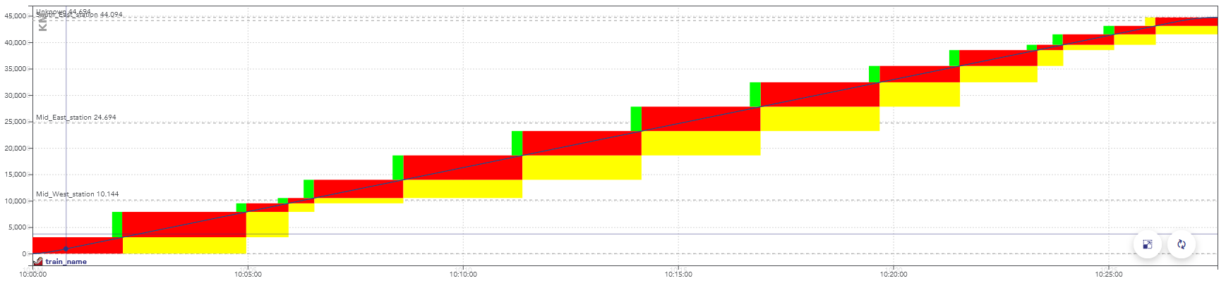
Example of a space-time chart displaying the passage of a train.
The colors here represent aspects of the signals, but display a consumption of the capacity as well: when these blocks overlap for two trains, they conflict.
There is a conflict between two trains when they reserve the same object at the same time, in incompatible configurations.
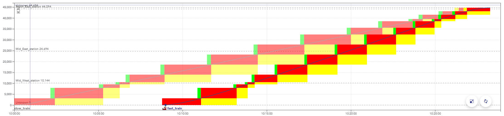
Example of a space-time graph with a conflict: the second train is faster than the first one, they are in conflict at the end of the path, when the rectangles overlap.
When simulating this timetable, the second train would be slowed down by the yellow signals, caused by the presence of the first train.
Train slots
A train slot corresponds to a capacity reservation for the passage of a train. It is fixed in space and time: the departure time and the path taken are known. On the space-time charts in this page, a train slot corresponds to the set of blocks displayed for a train.
Note: in English-speaking countries, these are often simply called “train paths”. But in this context, this name would be ambiguous with the physical path taken by the train.
The usual procedure is for the infrastructure manager (e.g. SNCF Réseau) to offers train slots for sale to railway companies (e.g. SNCF Voyageurs).
At a given date before the scheduled day of operation, all the train paths are allocated. But there may be enough capacity to fit more trains. Trains can fit between scheduled slots, when they are sufficiently far apart or have not found a buyer.
The remaining capacity after the allocation of train paths is called residual capacity. This section explains how OSRD looks for train slots in this residual capacity.
3.2.5.2 - Train slot search module
This module handles the search for solutions.
To summarize how it works: the search space is defined as one large decision tree.
We first build one decision tree that lists all possible paths, where each “decision” is the direction taken. We then build another tree on top of it that handles simulations and conflicts, branching is done when the new train gets to choose if it goes before or after a different train.
We then run an A* on the resulting graph.
3.2.5.2.1 - Infrastructure exploration
The first thing we need to define is how we move through the infrastructure, without dealing with conflicts yet.
We need a way to define and enumerate the different possible paths and explore the infrastructure graph, with several constraints:
- The path must be compatible with the given rolling stock (loading gauge / electrification / signaling system)
- At any point, we need to access path properties from its start up to the considered point. This includes block and route lists.
- We sometimes need to know where the train will go after the point currently being evaluated, for proper conflict detection
To do this, we have defined the class InfraExplorer.
It has one purpose: enumerating all possible paths.
This is the class that handles the “path” aspect of the decision tree.
It uses blocks (sections from signal to signal) as a main subdivision. It has 3 sections: the current block, predecessors, and a “lookahead”.

In this example, the green arrows are the predecessor blocks. What happens there is considered to be immutable.
The red arrow is the current block. This is where we run train and signaling simulations, and where we deal with conflicts.
The blue arrows are part of the lookahead. This section hasn’t
been simulated yet, its only purpose is to know in advance
where the train will go next. In this example, it would tell us
that the bottom right signal can be ignored entirely.
The top path is the path being currently evaluated.
The path that goes toward the bottom right track, if valid,
will be evaluated in a different InfraExplorer that would have
been generated alongside this instance.
The InfraExplorer is manipulated with two main functions
(the accessors have been removed here for clarity):
interface InfraExplorer {
    /**
     * Clone the current object and extend the lookahead by one route, for each route starting at
     * the current end of the lookahead section. The current instance is not modified.
     */
    fun cloneAndExtendLookahead(): Collection<InfraExplorer>

    /**
     * Move the current block by one, following the lookahead section. Can only be called when the
     * lookahead isn't empty.
     */
    fun moveForward(): InfraExplorer
}
cloneAndExtendLookahead() is the method that actually enumerates the
different paths, returning clones for each possibility.
It’s called when we need a more precise lookahead to properly identify
conflicts, or when it’s empty and we need to move forward.
A variation of this class can also keep track of the train simulation
and time information (called InfraExplorerWithEnvelope).
This is the version that is actually used to explore the infrastructure.
We now have a way to enumerate all possible paths:

3.2.5.2.2 - Conflict detection
Once we know what paths we can use, we need to know when they can actually be used.
The documentation of the conflict detection module explains how it’s done internally. Generally speaking, a train is in conflict when it has to slow down because of a signal. In our case, that means the solution would not be valid, we need to arrive later (or earlier) to see the signal when it’s not restrictive anymore.
In STDCM, conflicts can also be caused by work schedules.
The complex part is that we need to do the conflict detection incrementally Which means that:
- When running simulations up to t=x, we need to know all of the conflicts that happen before x, even if they’re indirectly caused by a signal seen at t > x down the path.
- We need to know the conflicts and resource uses right as they start even if their end time can’t be defined yet.
For that to be possible, we need to know where the train will go after the section that is being simulated (see infra exploration: we need some elements in the lookahead section).
To handle it, the conflict detection module returns an error when more lookahead is required. When it happens we extend it by cloning the infra explorer objects.
Note to maintainers: the actual incremental conflict detection is handled
by the class
IncrementalConflictDetector. When debugging in local,
it can be inspected and patched to identify exactly where requirements come from.3.2.5.2.3 - Conflict avoidance
While exploring the graph, it is possible to end up in locations that would generate conflicts. They can be avoided by adding delay.
Shifting the departure time
The departure time is defined as an interval in the module parameters:
the train can leave at a given time, or up to x seconds later.
Whenever possible, delay should be added by shifting the departure time.
for example : a train can leave between 10:00 and 11:00. Leaving at 10:00 would cause a conflict, the train actually needs to enter the destination station 15 minutes later. Making the train leave at 10:15 solves the problem.
In OSRD, this feature is handled by keeping track, for every edge, of the maximum duration by which we can delay the departure time. As long as this value is enough, conflicts are avoided this way.
This time shift is a value stored in every edge of the path. Once a path is found, the value is summed over the whole path. This is added to the departure time.
For example :
- a train leaves between 10:00 and 11:00. The initial maximum time shift is 1:00.
- At some point, an edge becomes unavailable 20 minutes after the train passage. The value is now at 20 for any edge accessed from here.
- The departure time is then delayed by 5 minutes to avoid a conflict. The maximum time shift value is now at 15 minutes.
- This process is applied until the destination is found, or until no more delay can be added this way.
Engineering allowances
Once the maximum delay is at 0, the delay needs to be added between two points of the path.
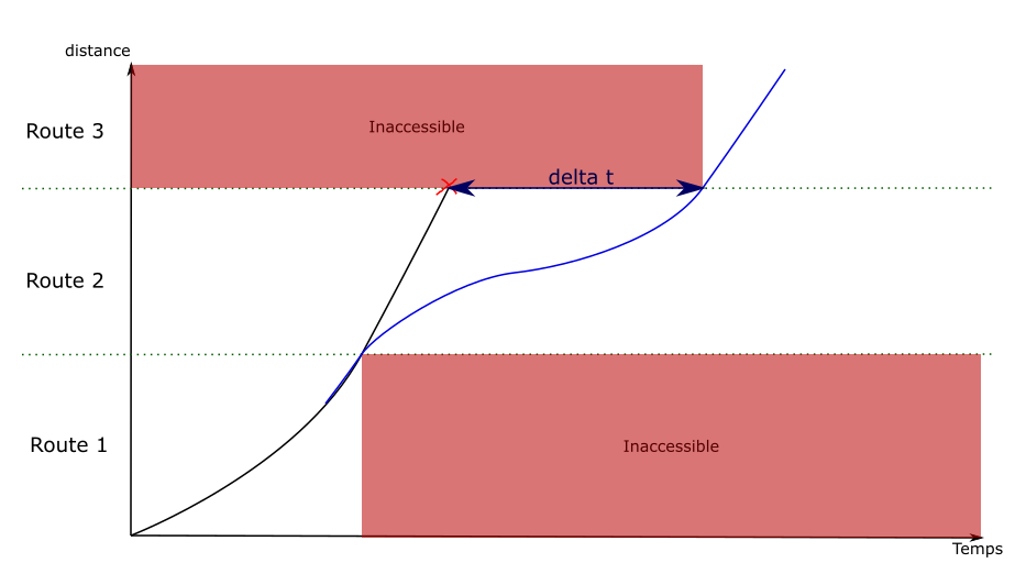
The idea is the same as the one used to fix speed discontinuities: new edges are created, replacing the previous ones. The new edges have an engineering allowance, to add the delay where it is possible.
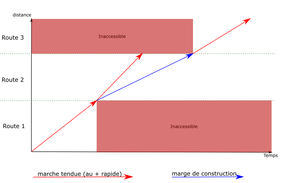
computing an engineering allowance is a feature of the running-time calculation module. It adds a given delay between two points of a path, without affecting the speeds on the rest of the path.
Post-processing
We used to compute the engineering allowances during the graph exploration, but that process was far too expensive. We used to run binary searches on full simulations, which would sometimes go back for a long distance in the path.
What we actually need is to know whether an engineering allowance is possible without causing any conflict. We can use heuristics here, as long as we’re on the conservative side: we can’t say that it’s possible if it isn’t, but missing solutions with extremely tight allowances isn’t a bad thing in our use cases.
But this change means that, once the solution is found, we can’t simply concatenate the simulation results. We need to run a full simulation, with actual engineering allowances, that avoid any conflict. This step has been merged with the one described on the standard allowance page, which is now run even when no standard allowance have been set.
3.2.5.2.4 - Discontinuities and backtracking
The discontinuity problem
When a new graph edge is visited, a simulation is run to evaluate its speed. But it is not possible to see beyond the current edge. This makes it difficult to compute braking curves, because they can span over several edges.
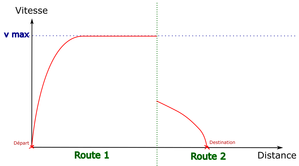
This example illustrates the problem: by default the first edge is explored by going at maximum speed. The destination is only visible once the second edge is visited, which doesn’t leave enough distance to stop.
Solution : backtracking
To solve this problem, when an edge is generated with a discontinuity in the speed envelopes, the algorithm goes back over the previous edges to create new ones that include the decelerations.
To give a simplified example, on a path of 4 edges where the train can accelerate or decelerate by 10km/h per edge:
![]()
For the train to stop at the end of route 4, it must be at most at 10km/h at the end of edge 3. A new edge is then created on edge 3, which ends at 10km/h. A deceleration is computed backwards from the end of the edge back to the start, until the original curve is met (or the start of the edge).
In this example, the discontinuity has only been moved to the transition between edges 2 and 3. The process is then repeated on edge 2, which gives the following result:
![]()
Old edges are still present in the graph as they can lead to other solutions.
3.2.5.2.5 - Search space and decision tree
Now that we can enumerate the paths and identify conflicts, we need to build the final decision tree that avoids all conflicts.
In terms of implementation, we would like to have a class with a similar
purpose as
InfraExplorer, but currently it’s all over the place.
There’s a refactoring issue,
but we may not have the time to do it.The search space is described as a graph with nodes and edges. Edges are generally one signaling block long, but may be shorter in case of stops.
Generating new edges on a given path follow this sequence:
- The train movement is generated on the new segment (time and speed at each point)
- Conflicts are identified during this time segment
- Openings are identified
- One edge is generated per opening
An “opening” is an available time window between two occupied blocks. When there are several different openings, we get to choose if the new train goes before or after another train or work schedule.
On one given path, we now have a decision tree that looks like this:

Delays
We often need to add delay to the current simulation to actually go through an opening, when the train needs to reach a point later than it could have.
This can be done in several different ways:
- Delaying the train departure
- Lengthening a stop
- Forcing the train to go slower for a while (with something called “engineering allowances”)
We keep track of how much delay we can add at any given point to handle departure and stop changes. For engineering allowances, we’re identifying how much delay we can add if the train slows down then immediately speeds up.
3.2.5.2.6 - The actual pathfinding
Once we have a graph that describes the entire search space, we can run a pathfinding algorithm. In this case, we use an A*.
We need to define a few things first:
- How to sort the nodes, which defines which solution is considered better than the other
- How to identify redundant nodes
- How to estimate the remaining “cost” at any given point (the heuristic)
Node ordering
We currently define a hierarchy across different criteria: we first compare the most important one, and move on to the next if equal, until we reach the end of the list.
That order is defined in STDCMNode,
in compareTo. It tends to change more often than this website
is updated, so it’s best to check the code itself.
The main criteria is the best possible total travel time: the sum of the current travel time to reach this node and the minimum remaining travel time from this node to the destination (as defined/computed by the heuristic). Stop duration isn’t included here.
Defining redundant (visited) nodes
This is handled by VisitedNodes.
The idea is that, at any given physical location, we mark time ranges as “visited”.
For example: consider a node reached at earliest t=10:00, where we can delay the departure by 30 minutes, and we can’t add any engineering allowance (added time by slowing down). Then the location will be flagged as “visited” from t=10:00 to t=10:30.
Engineering allowance means we can also reach some other time range by lengthening the travel time. But it may not be the optimal way to reach a given time. So we can mark a range as “conditionally visited”, where it’s visited at a given cost value. These ranges are compared to the new range and cost to identify if the new node is redundant.
Heuristic
Most of the algorithmic complexity here comes from the high number of nodes for any given location. Going through the entire block graph once is comparatively quite fast.
So we go through the entire block graph, starting at the destination, and we keep track of the fastest time it takes to reach the destination from any given point.
We keep track of intermediate path steps, max speed, and decelerations (including decelerations caused by requested stops). But we can’t consider accelerations at this stage.
It may sound slow and expensive (and it can be), but it drastically lowers the standard deviation and upper bound in search time.
3.2.5.2.7 - Standard allowance
The STDCM module must be usable with standard allowances. The user can set an allowance value, expressed either as a function of the running time or the travelled distance. This time must be added to the running time, so that it arrives later compared to its fastest possible running time.
For example: the user can set a margin of 5 minutes per 100km. On a 42km long path that would take 10 minutes at best, the train should arrive 12 minutes and 6 seconds after leaving.
This can cause problems to detect conflicts, as an allowance would move the end of the train slot to a later time. The allowance must be considered when we compute conflicts as the graph is explored.
The allowance should also follow the MARECO model: the extra time isn’t added evenly over the whole path, it is computed in a way that requires knowing the whole path. This is done to optimize the energy used by the train.
During the exploration
The main implication of the standard allowance is during the graph exploration, when we identify conflicts. It means that we need to scale down the speeds. We still need to compute the maximum speed simulations (as they define the extra time), but when identifying at which time we see a given signal, all speeds and times are scaled.
This process is not exact. It doesn’t properly account for the way the allowance is applied (especially for MARECO). But at this point we don’t need exact times, we just need to identify whether a solution would exist at this approximate time.
This slightly inexact process may seem like a problem, but in
reality (for SNCF) standard allowances actually have some
tolerance between arbitrary points on the path. e.g. if
we should aim for 5 minutes per 100km, any value between
3 and 7 would be valid. The actual tolerance is not something
we can or want to encode as they’re too many specificities,
but it means we can be off by a few seconds.
Post-processing
The process to find the actual train simulation is as follows:
- We define points at which the time is fixed, initialized at first with the time of each train stop. This is an input of the simulation and indirectly calls the standard allowance.
- We run a full simulation over the entire path with conflict detection
- If there are conflicts, we try to remove the first one.
- We add a fixed time point at the location where that conflict happened. We use the time considered during the exploration (with linear scaling) as reference time.
- This process is repeated iteratively until no conflict is found.
This is the general idea. In practice, we need some workarounds to avoid some issues. These include:
- Adding a fixed time point at the end location of engineering allowances (when not part of a different engineering allowance)
- Distributing engineering allowance times linearly over the engineering allowance distance
- When we fail to find a valid solution, we fall back from MARECO to “linear” allowance distribution
- When we still fail to find a valid solution, we increase the train traction. This lets us find a close solution.
When we fail to find a solution despite all this, an error is thrown and needs to be investigated. It can be difficult to identify what went wrong though, it can come from any difference and mismatch between the search and this final post-processing simulation.
3.2.5.2.8 - Implementation details and current issues
This page is about implementation details. It isn’t necessary to understand general principles, but it helps before reading the code.
STDCMEdgeBuilder
This refers to this class in the project.
This class is used to make it easier to create instances of
STDCMEdge, the graph edges. These contain many attributes,
most of which can be determined from the context (e.g. the
previous node).
The STDCMEdgeBuilder class makes some parameters optional
and automatically computes others.
Once instantiated and parameterized, an STDCMEdgeBuilder has two methods:
makeAllEdges(): Collection<STDCMEdge>can be used to create all the possible edges in the given context for a given route. If there are several “openings” between occupancy blocks, one edge is instantiated for each opening. Every conflict, their avoidance, and their related attributes are handled here.findEdgeSameNextOccupancy(double timeNextOccupancy): STDCMEdge?: This method is used to get the specific edges that uses a certain opening (when it exists), identified here with the time of the next occupancy block. It is called whenever a new edge must be re-created to replace an old one. It calls the previous method.
Note: ideally, we would have a class similar to
InfraExplorer
that would just enumerate all possible simulations. It would be
much cleaner than this current state. See this issue.Past path data
During the exploration, we simulate each block on its own, ignoring where the train comes from. This is done to improve caching, and because past path data is currently difficult to fetch.
This has two issues:
- We need to consider that speed limits apply until the train head leaves the speed limit range. This is technically wrong, it should be dismissed when the train tail leaves it.
- During the search, we don’t know the slopes on the tracks still covered by the train. This can lead to accelerations that are too optimistic, and in rare cases to post-processing errors.
There’s an open issue, but we don’t have a clear plan nor the time to work on it (yet).
3.2.6 - Timetable v2
Describes evolutions to the new timetable and train schedule models

Design decisions
Some major changes were made between our first version of the timetable and the new one:
- Isolate the timetable table. It can be used in a scenario or in other contexts
- Have a soft reference from train schedule to rolling stock (to be able to create a train schedule with unknown rolling stock)
- Consider path and simulation output as cache (that don’t require to be stored in DB)
- We can compute pathfinding without having to store data
- All input needed to compute a path is stored in the train schedule (we can recompute it if needed)
- All input needed to run a simulation is stored in the train schedule (we can recompute it if needed)
Train schedule v2
Requirements
front: easy to keep consistent during editionfront: intermediate invalid states than can be reached during edition have to be encodableimport: path waypoint locations can be specified using UIC operational point codesimport: support fixed scheduled arrival times at stops and arbitrary pointsimportedition: train schedules must be self-contained: they cannot be described using the result of pathfinding or simulations
Design decisions
Path waypoints have an identity
At some point in the design process, the question was raised of whether to reference location of stops and margin transitions by name, or by value. That is, should stops hold the index of the waypoint where the stop occurs, or a description of the location where the stop occurs?
It was decided to add identifiers to path waypoints, and to reference those identifiers where referencing a path location is needed. This has multiple upsides:
- you can’t reference a location outside of the path
- when changing a waypoint’s location, for example from one station’s platform to another, no additional work is needed to keep the path consistent
- if a path goes to the same place multiple times, the identifier reference makes it clear which path location is referenced
- it makes keeping data consistent while editing easier, as all locations are kept in a single place
Separating path and stops
This decision was hard to make, as there are little factors influencing this decision. Two observations led us to this decision:
- when deleting a waypoint, the end user may want to preserve the associated stop. Making the separation clear in the data model helps with implementing this behavior correctly, if deemed relevant
- bundling stops into the path makes it harder to describe what fields
pathwaypoints should have, and what should have a separate object and reference. It was decided that keepingpatha simple list ofLocation, with no strings attached, made things a little clearer.
No more engineering margins?
In the legacy model, we had engineering margins. These margins had the property of being able to overlap. It was also possible to choose the distribution algorithm for each margin individually.
We asked users to comment on the difference and the usefulness of retaining these margins with scheduled points. The answer is that there is no fundamental difference, and that the additional flexibility offered by engineering margins makes no practical sense (overlap and choice of distribution…).
Arrival times are durations since departure time
- this allows shifting the departure time without having to change arrival times
- we don’t have to parse dates and compute date differences within a single trip
We also discussed whether to use seconds or ISO 8601 durations. In the end, ISO 8601 was chosen, despite the simplicity of seconds:
- it preserves the user’s choice unit for specifying duration
- it interfaces nicely with the ISO 8601 departure time
- it does not suffer from potential integer-float serialization related precision loss
Invalid and outdated train schedules
Reasons for a train schedule to be invalid:
- Rolling stock not found
- Path waypoint not found
- The path cannot be found
Reasons for a train schedule to be outdated:
- The train path changed
- The train running time changed
What we can do about outdated trains:
- Nothing, they’re updated without notification
- We can notify the user that a train schedule is outdated:
- Nothing can be done except acknowledge the change
- We can not check what changed between the old and new version
- We can not know the cause of this change (RS, Infra, Algorithms…)
Note: The outdated status is a nice to have feature (it won’t be implemented right now).
Creation fields
These fields are required at creation time, but cannot be changed afterwards. They are returned when the train schedule is queried.
timetable_id: 42
Modifiable fields
train_name: "ABC3615"
rolling_stock_name: R2D2

# labels are metadata. They're only used for display filtering
labels: ["tchou-tchou", "choo-choo"]

# used to select speed limits for simulation
speed_limit_tag: "MA100"

# the start time is an ISO 8601 datetime with timezone. it is not always the
# same at the departure time, as there may be a stop at the starting point
start_time: "2023-12-21T08:51:11.914897+00:00"

path: # Either a “track and offset”, or an “operational point and an optional local track name”
 - {id: a, uic: 87210, local_track_name: "V1"} # Any operational point matching the given uic
 - {id: b, track: foo, offset: 10000} # 10m on track foo
 - {id: c, trigram: ABC} # Any operational point matching the trigram ABC
 - {id: d, operational_point: X} # A specified operational point

# the algorithm used for distributing margins and scheduled times
constraint_distribution: MARECO # or LINEAR

# all durations and times are specified using ISO 8601
# we don't supports months and years duration since it's ambiguous
# times are defined as time elapsed since start. Even if the attribute is omitted,
# a scheduled point at the starting point is inferred to have departure=start_time
#
# To specify signal's state on stop's arrival, you can use the "reception_signal" enum:
#   - OPEN: arrival on open signal, will reserve resource downstream of the signal.
#   - STOP: arrival on stop signal, will not reserve resource downstream of the signal
#      and will trigger safety speed on approach.
#   - SHORT_SLIP_STOP: arrival on stop signal with a short slip distance,
#      will not reserve resource downstream of the signal and will trigger safety
#      speed on approach as well as short slip distance speed.
#      This is used for cases where a movable element is placed shortly after the signal
#      and going beyond the signal would cause major problems.
#      This is used automatically for any stop before a buffer-stop.
#      This is also the default use for STDCM stops, as it is the most restrictive.
schedule:
 - {at: a, stop_for: PT5M} # inferred arrival to be equal to start_time
 - {at: b, arrival: PT10M, stop_for: PT5M}
 - {at: c, stop_for: PT5M}
 - {at: d, arrival: PT50M, reception_signal: SHORT_SLIP_STOP}

margins:
  # This example encodes the following margins:
  #   a --- 5% --- b --- 3% --- c --- 4.5min/100km --- d

  # /!\ all schedule points with either an arrival or departure time must also be
  # margin boundaries. departure and arrival waypoints are implicit boundaries. /!\
  # boundaries delimit margin sections. A list of N boundaries yields N + 1 sections.
  boundaries: [b, c]

  # the following units are supported:
  #  - % means added percentage of the base simulation time
  #  - min/100km means minutes per 100 kilometers
  values: ["5%", "3%", "4.5min/100km"]

# train speed at simulation start, in meters per second.
# must be zero if the train starts at a stop
initial_speed: 2.5

power_restrictions:
 - {from: b, to: c, value: "M1C1"}

comfort: AIR_CONDITIONING # or HEATING, default STANDARD

options:
  # Should we use electrical profiles to select rolling stock speed effort curves
  use_electrical_profiles: true

# Category defines the type of train.
# It can be either a predefined main category (like high-speed or freight),
# or a custom sub-category referenced by its code.
# Only one of the two options must be provided.
category:
  main_category: "HIGH_SPEED_TRAIN"

# or sub category code
category:
  sub_category_code: "RER"
Combining margins and schedule
Margins and scheduled points are two ways to add time constraints to a train’s schedule. Therefore, there must be a clear set of rules to figure out how these two interfaces interact.
The end goal is to make the target schedule and margins consistent with each other. This is achieved by:
- computing what the schedule would look like if only margins were applied
- compare that to the target schedule
- correct the margin schedule so that it matches the target schedule
The path is partitioned as follows:
- known time sections span between locations where the arrival time is known.
If there are
Nsuch locations, there areN - 1known time sections. In these sections, margins need to be adjusted to match the target schedule. - If the arrival time at destination is unknown, the section from the last known arrival time point and the destination is called the relaxed time section has no bound. Margins can be applied directly.
As margins cannot span known time section boundaries, each known time section can be further subdivided into margin sections. Margins cover the entire path.
The end goal is to find the target arrival time at the end of each margin section. This needs to be done while preserving consistency with the input schedule.

Note that stops do not impact margin repartition. For example, the margin does not need to be proportionally distributed on each side of b.
The same goes for points with arrival time. They impact whether the margin is respected or not, but they do not force the margin to be proportionally distributed on each side of the point.
The final schedule is computed as follows:
- A base simulation is computed, without any time constraint (other than stops). It’s used to compute provisional margin values.
- Make a provisional time table, which ignores target arrival times but includes provisional margin values.
- For each known time section, compute the adjustment required to make the provisional schedule match the target schedule.
- Distribute this difference into the known time section’s margin sections, proportionally to margin section running time. After distributing the adjustment into margin sections, the final schedule should be compatible with the target schedule.
Error handling
Some errors may happen while building the timetable:
- if a known time section’s required adjustment is negative, a warning must be raised, as margins will have to be lowered
- if a margin section’s final running time is tighter than the base simulation, it cannot be achieved, and a warning should be raised
Other errors can happen at runtime:
- target margin values can be too low, as transitions from high density margin to low margin section force the train to lose time after it has exited to high density margin section.
- target margin values can also be too high, as the train may not have time to slow down enough, or drive so slow as to be unacceptable.
During simulation, if a target arrival time cannot be achieved, the rest of the schedule still stands.
Paced Train
The Paced Train in OSRD is a way to generate multiple trains at regular intervals over a defined time window.
It extends a standard TrainSchedule with the following additional fields:
- interval: Duration (ISO 8601) – the time between two consecutive trains (e.g., PT15M for one train every 15 minutes).
- time_window: Duration (ISO 8601) – the total duration during which the trains are repeated (e.g., PT1H for a total of 1 hour).
- exceptions: List of exceptions
paced:
  interval: "PT30M"
  time_window: "PT1H"
exceptions: []
Example
- start_time = 08:00
- interval = PT15M
- time_window = PT1H
A mission with a step of 15 min and a duration of 1 hour will see 4 trains running from the departure time. This will generate four base trains at 08:00, 08:15, 08:30, and 08:45.
Exceptions
Paced Trains support exceptions, which allow modifying the base schedule in flexible ways. Each exception is identified by a unique key and can be of the following types:
- Modified: changes a specific base occurrence (e.g., change the train name or start time at index 2).
- Created: adds a new train outside the regular base schedule (e.g., an extra train at 08:10).
- Disabled: allows disabling the effect of an occurrence.
Modified exceptions:
A modified exception alters an occurrence generated from the interval-based schedule.
- Identified by the presence of the occurrence_index field.
- Can include one or more change groups to override train schedule properties.
- Requires a unique key.
- Can be disabled using the disabled flag.
key: "exception_1"
occurrence_index: 1
disabled: false
# changes groups
Created exceptions
Created exceptions are user-defined exceptions that add a new train outside the occurrences generated from the intervals. They are distinguished by the absence of the occurrence_index field.
key: "exception_2"
disabled: false
# changes groups
Change Groups
Each exception can optionally include one or more change groups. A change group represents a structured override for part of the train schedule.
- If a change group is not present, the value from the base schedule is used.
- If a field is provided in the change group but left empty, the corresponding field in the schedule will be unset.
- Otherwise, the change group’s value will override the base schedule.
See train schedule modifiable fields for more details
train_name:
  value: "New Train Name" # Override the train's name

rolling_stock:
  rolling_stock_name: "R2D2"
  comfort: "STANDARD" # Override rolling stock and comfort class

rolling_stock_category:
  value:
    main_category: "HIGH_SPEED_TRAIN" # Override the train main category
    # OR (mutually exclusive)
    sub_category_code: "RER" # Override the sub category (e.g., RER)

labels:
  value: ["tchou-tchou", "choo-choo"]

speed_limit_tag:
  value: "MA100"

start_time:
  value: "2024-05-22T08:10:00Z" # Override the train’s departure time

constraint_distribution:
  value: "MARECO" # Override planning constraints (e.g., safety margins)

initial_speed:
  value: 2.5 # Override the initial speed in m/s

options:
  value:
    use_electrical_profiles: false

path_and_schedule: # Override path, schedule, margins and power_restrictions fields
  path:
  schedule:
  margins:
  power_restrictions:
Endpoints
Timetable
POST /timetable
GET /timetable/ # Paginated list timetable
PUT /timetable/ID
DELETE /timetable/ID
GET /timetable/ID/train_schedules # Paginated list of train schedules
GET /timetable/ID/paced_trains # Paginated list of paced_trains
Train Schedule
POST /timetable/ID/train_schedules # A batch creation
GET /train_schedule/ID
PUT /train_schedule/ID # Update a specific train schedule
DELETE /train_schedule # A batch deletion
Paced Train
POST /timetable/ID/paced_trains # A batch creation
GET /paced_train/ID
PUT /paced_train/ID # Update a specific paced train
DELETE /paced_trains # A batch deletion
Path
POST /infra/ID/pathfinding/topo # Not required now can be move later
POST /infra/ID/pathfinding/blocks
# takes a pathfinding result and a list of properties to extract
POST /infra/ID/path_properties?props[]=slopes&props[]=gradients&props[]=electrifications&props[]=geometry&props[]=operational_points
GET /train_schedule/ID/path?infra_id=42 # Retrieve the path from a train schedule
GET /paced_train/ID/path?infra_id=42 # Retrieve the path from a paced_train
Simulation results
# Retrieve the list of conflict of the timetable (invalid trains are ignored)
GET /timetable/ID/conflicts?infra=N
# Retrieve the space, speed and time curve of a given train
GET /train_schedule/ID/simulation?infra=N
# Retrieve the space, speed and time curve of a given paced train
GET /paced_train/ID/simulation?infra=N
# Retrieves simulation information for a given train list. Useful for finding out whether pathfinding/simulation was successful.
GET /train_schedule/simulations_summary?infra=N&ids[]=X&ids[]=Y
# Retrieves simulation information for a given paced train list. Useful for finding out whether pathfinding/simulation was successful.
GET /paced_train/simulations_summary?infra=N&ids[]=X&ids[]=Y
# Projects the space time curves and paths of a number of train schedules onto a given path
POST /v2/train_schedule/project_path?infra=N&ids[]=X&ids[]=Y
# Projects the space time curves and paths of a number of paced trains onto a given path
POST /paced_train/project_path?infra=N&ids[]=X&ids[]=Y
Frontend workflow
The frontend shouldn’t wait minutes to display something to the user. When a timetable contains hundreds of trains it can take some time to simulate everything. The idea is to split requests into small batches.
flowchart TB
    InfraLoaded[Check for infra to be loaded]
    RetrieveTimetable[Retrieve Timetable]
    RetrieveTrains[Retrieve TS2 payloads]
    SummarySimulation[[Summary simulation batch N:N+10]]
    TrainProjectionPath[Get selected train projection path]
    Projection[[Projection batch N-10:N]]
    TrainSimulation[Get selected train simulation]
    TrainPath[Get selected train path]
    TrainPathProperties[Get selected train path properties]
    DisplayGev(Display: GEV / Map /\n Driver Schedule/ Linear / Output Table)
    DisplayGet(Display Space Time Chart)
    DisplayTrainList(Display train list)
    Conflicts(Compute and display conflicts)
    ProjectConflicts(Display conflicts in GET)


    InfraLoaded -->|Wait| SummarySimulation
    InfraLoaded -->|Wait| TrainProjectionPath
    InfraLoaded -->|Wait| TrainPath
    TrainPath -->|If found| TrainSimulation
    TrainPath -->|If found| TrainPathProperties
    RetrieveTimetable -->|Get train ids| RetrieveTrains
    RetrieveTrains ==>|Sort trains and chunk it| SummarySimulation
    SummarySimulation ==>|Wait for the previous batch| Projection
    SummarySimulation -->|Gradually fill cards| DisplayTrainList
    TrainPathProperties -->| | DisplayGev
    TrainSimulation -->|If valid simulation| DisplayGev
    TrainProjectionPath -->|Wait for the previous batch| Projection
    SummarySimulation -..->|If no projection train id| TrainProjectionPath
    Projection ==>|Gradually fill| DisplayGet
    SummarySimulation -->|Once everything is simulated| Conflicts
    Conflicts --> ProjectConflicts
3.2.7 - Authentication and authorization
Context and requirements
- authentication (
authn) is the process of figuring out a user’s identity. - authorization (
authz) is the process of figuring out whether a user can do something.
This design project started as a result of a feature request coming from SNCF users and stakeholders. After some interviews, we believe the overall needs to be as follows:
- controlling access to features
- some users are supposed to only view results of operational studies
- some users only get access to part of the app
- not everyone can have access to the admin panel
- it could be nice to be able to roll experimental features out incrementally
- controlling access to data
- some infrastructures shall only be changed by automated import jobs
- users might want to control who can mess with what they’re currently working on
- rolling stock, infrastructure and timetable data may be confidential
Overall architecture
flowchart LR
  subgraph gateway
    auth([authentication])
  end

  subgraph editoast
  subgraph authorization
    roles([role check])
    permissions([permission check])
  end
  end

  subgraph decisions
    permit
    deny
  end

  request --> auth --> roles --> permissions
  auth --> deny
  roles --> deny
  permissions --> permit & deny
Authentication
The app’s backend is not responsible for authenticating the user: it gets all required information
from gateway, the authenticating reverse proxy which stands between it and the front-end.
- at application start-up, the front-end redirects to the login page if the user is not logged in
- if the user is already authenticated, the gateway returns user metadata
- otherwise, the gateway initiates the authentication process, usually with OIDC. The implementation was designed to allow new backends to be added easily.
- once the user is authenticated, all requests to the backend can expect the following headers to be set:
x-remote-user-identitycontain a unique identifier for this identity. It can be thought of as an opaqueprovider_id/user_idtuple.x-remote-user-namecontain a username
When editoast receives a request, it has to match the remote user ID with a database user, creating it as needed.
create table authn_subject(
  id  bigserial generated always as identity primary key,
);

create table authn_user(
  id  bigint primary key references auth_subject on delete cascade,
  identity_id  text not null,
  name  text,
);

create table authn_group(
  id bigint primary key references auth_subject on delete cascade,
  name text not null,
);

-- add a trigger so that when a group is deleted, the associated authn_subject is deleted too
-- add a trigger so that when a user is deleted, the associated authn_subject is deleted too

create table authn_group_membership(
  user   bigint references auth_user  on delete cascade not null,
  group  bigint references auth_group on delete cascade not null,
  unique (user, group),
);
Group and role management API
Users cannot be directly created. The authenticating reverse proxy is in charge of user management.
- role management is protected by the
role:adminrole. - groups management is subject to permissions.
Get information about a user
GET /authn/me
GET /authn/user/{user_id}
{
  "id": 42,
  "name": "Foo Bar",
  "groups": [
    {"id": 1, "name": "A"},
    {"id": 2, "name": "B"}
  ],
  "app_roles": ["ops"],
  "builtin_roles": ["infra:read"]
}
Builtin roles are deduced from app roles, and thus cannot be directly edited.
Add roles to a user or group
This endpoint can only be called if the user has the role:admin builtin role.
POST /authn/user/{user_id}/roles/add
POST /authn/group/{group_id}/roles/add
Takes a list of app roles:
["ops", "stdcm"]
Remove roles from a user or group
This endpoint can only be called if the user has the role:admin builtin role.
POST /authn/user/{user_id}/roles/remove
Takes a list of app roles to remove:
["ops"]
Create a group
This endpoint can only be called if the user has the group:create builtin role.
When a user creates a group, it becomes its owner.
POST /authn/group
{
  "name": "Foo"
  "app_roles": ["ops"],
}
Returns the group ID.
Add users to a group
Can only be called if the user has Writer access to the group.
POST /authn/group/{group_id}/add
Takes a list of user IDs
[1, 2, 3]
Remove users from a group
Can only be called if the user has Writer access to the group.
POST /authn/group/{group_id}/remove
Takes a list of user IDs
[1, 2, 3]
Delete a group
Can only be called if the user has Owner access to the group.
DELETE /authn/group/{group_id}
Authorization
As shown in the overall architecture section, to determine if a subject is allowed to conduct an action on a resource, two checks are performed:
- We check that the roles of the subject allows the action.
- We check that the subject has the minimum privileges on the resource(s) that are required to perform the action.
Roles
Subject can have any number of roles. Roles allow access to features. Roles do not give rights on specific objects.
Both the frontend and backend require some roles to be set to allow access to parts of the app. In the frontend, roles guard features, in the backend, roles guard endpoints or group of endpoints.
There are two types of roles:
- Builtin roles are bundled with OSRD. Only builtin roles can be required by endpoints. These roles cannot directly be assigned to users.
- Application roles can be assigned to users. These roles are defined in a configuration file that editoast reads at startup.
Here is an example of what builtin roles might look like:
role:adminallows assigning roles to users and groupsgroup:createallows creating user groupsinfra:readallows access to the map viewer moduleinfra:writeimpliesinfra:read. it allows access to the infrastructure editor.rolling-stock:readrolling-stock:writeimpliesrolling-stock:read. Allows access to the rolling stock editor.timetable:readtimetable:writeimpliestimetable:readoperational-studies:readallows read only access to operational studies. it impliesinfra:read,timetable:readandrolling-stock:readoperational-studies:writeallows write access to operational studies. it impliesoperational-studies:readandtimetable:writestdcmimpliesinfra:read,timetable:readandrolling-stock:read. it allows access to the short term path request module.admingives access to the admin panel, and implies all other roles
Given these builtin roles, application roles may look like:
operational-studies-customerimpliesoperational-studies:readoperational-studies-analystimpliesoperational-studies:writestdcm-customerimpliesstdcmopsimpliesadmin
Roles are hierarchical. This is a necessity to ensure that, for example, if we are to introduce a new action related to scenarios, each subject with the role “exploitation studies” gets that new role automatically. We’d otherwise need to edit the appropriate existing roles.
Their hierarchy could resemble:
%%{init: {"flowchart": {"defaultRenderer": "elk"}} }%%
flowchart TD
  subgraph application roles
    operational-studies-analyst
    operational-studies-customer
  end

  subgraph builtin roles
    rolling-stock:read
    rolling-stock:write
    infra:read
    infra:write
    timetable:read
    timetable:write
    operational-studies:read
    operational-studies:write
  end

  operational-studies-analyst --> operational-studies:write
  operational-studies-customer --> operational-studies:read

  infra:write --> infra:read
  rolling-stock:write --> rolling-stock:read
  operational-studies:read --> infra:read & timetable:read & rolling-stock:read
  operational-studies:write --> operational-studies:read & timetable:write
  timetable:write --> timetable:read

  classDef app fill:#333,color:white,font-style:italic
  classDef builtin fill:#992233,color:white,font-style:bold

  class stdcm,exploitation,infra,project,study,scenario app
  class infra_read,infra_edit,infra_delete,project_create,study_delete,scenario_create,scenario_update builtin
Permissions
Permission checks are done by the backend, even though the frontend may use the effective privilege level of a user to decide whether to allow modifying / changing permissions for a given object.
Permissions are checked per resource, after checking roles. A single request may involve multiple resources, and as such involve multiple permission checks.
Permission checks are performed as follows:
- for each request, before any resource is accessed, compute which resources need access and required privilege levels
- figure out, for the request’s user, its effective privilege level for every involved resource
- if the user’s privilege level does not meet expectations, raise an error before any change is made
enum EffectivePrivLvl {
    Owner,    // all operations allowed, including granting access and deleting the resource
    Writer,   // can change the resource
    Creator,  // can create new sub resources
    Reader,   // can read the resource
    MinimalMetadata, // is indirectly aware that the resource exists
}

trait Resource {
    #[must_use]
    fn get_privlvl(resource_pk: u64, user: &UserIdentity) -> EffectivePrivLvl;
}
The backend may therefore perform one or more privilege check per request:
- pathfinding:
Readeron the infrastructure
- displaying a timetable:
Readeron each rolling stock
- batch train creation:
Creatoron the timetable
- conflict detection:
Readeron the infrastructureReaderon the timetableReaderon every involved rolling stock
- simulation results:
Readeron the infrastructureReaderon the rolling stock
A grant is a right, given to a user or group on a specific resource. Users get privileges through grants. There are two types of grants:
- explicit grants are explicitly attached to resources
- implicit grants automatically propagate explicit grants for objects which belong to a hierarchy:
- if a subject owns a project, it also owns all studies and scenarios
- if a subject can read a scenario, it knows the parent study and project exist
Explicit grants
- can be edited from the frontend
- any user holding grants over a resource can add new ones
- when a resource is created,
Owneris granted to the current user - not all objects type can have explicit grants: train schedule inherit their timetable’s grants
-- this type is the same as EffectivePrivLvl, except that MinimalMetadata is absent,
-- as it cannot be granted directly. mere knowledge that an object exist can only be
-- granted using implicit grants.
create type grant_privlvl as enum ('Owner', 'Writer', 'Creator', 'Reader');

-- this table is a template, which other grant tables are
-- designed to be created from. it must be kept empty.
create table authz_template_grant(
  -- if subject is null, this grant applies to any subject
  subject     bigint references authn_subject on delete cascade,
  grant       grant_privlvl not null,
  granted_by  bigint references authn_user on delete set null,
  granted_at  timestamp not null default CURRENT_TIMESTAMP,
);
-- these indices speed up cascade deletes
create index on authz_template_grant(subject);
create index on authz_template_grant(granted_by);

-- create a new grant table for infrastructures
create table authz_grant_EXAMPLE (
  like authz_template_grant including all,
  resource bigint references EXAMPLE on delete cascade not null,
  unique nulls not distinct (resource, subject),
);

-- raise an error if grants are inserted into the template
create function authz_grant_insert_error() RETURNS trigger AS $err$
    BEGIN
        RAISE EXCEPTION 'authz_grant is a template, which other grant '
        'tables are designed to inherit from. it must be kept empty.';
    END;
$err$ LANGUAGE plpgsql;
create trigger before insert on authz_template_grant execute function authz_grant_insert_error();
Implicit grants
Implicit grants only apply to the operational studies module, not timetables, infrastructures and rolling stocks.
Implicit grants propagate explicit grants to related objects. There are two types of implicit grants:
- explicit grants propagate downwards within hierarchies:
Owner,Reader,Writerpropagate as is,Creatoris reduced toReader MinimalMetadatapropagates up within project hierarchies, so that read access to a study or scenario allows having the name and description of the parent project
The following objects have implicit grants:
projectgetsMinimalMetadataif the user has any right on a child study or scenariostudygets:MinimalMetadataif the user has any right on a child scenarioOwner,Reader,Writerif the user has such right on the parent study.Creatoris reduced toReader.
scenariogetsOwner,Reader,Writerif the user has such right on the parent study or project.Creatoris reduced toReader.train-schedules have the same grants as their timetable
Permission meta-model
Get the privilege level of the current user
GET /authz/{resource_type}/{resource_id}/privlvl
Get all grants for a resource
GET /authz/{resource_type}/{resource_id}/grants
[
  {
    "subject": {"kind": "group", "id": 42, "name": "Bar"},
    "implicit_grant": "Owner",
    "implicit_grant_source": "project"
  },
  {
    "subject": {"kind": "user", "id": 42, "name": "Foo"},
    "grant": "Writer"
  },
  {
    "subject": {"kind": "user", "id": 42, "name": "Foo"},
    "grant": "Writer",
    "implicit_grant": "MinimalMetadata",
    "implicit_grant_source": "project"
  }
]
Implicit grants cannot be edited, and are only displayed to inform the end user.
Add a new grant
POST /authz/{resource_type}/{resource_id}/grants
{
  "subject_id": 42,
  "grant": "Writer"
}
Change a grant
PATCH /authz/{resource_type}/{resource_id}/grants/{grant_id}
{
  "grant": "Reader"
}
Revoke a grant
DELETE /authz/{resource_type}/{resource_id}/grants/{grant_id}
Implementation plan
Phase 1: ground work
Back-end:
- pass the proper headers from the reverse proxy to editoast
- implement the authn / authz model into the database
- get / create users on the fly using reverse proxy headers
- implement the role parsing and book-keeping (it can be parsed on startup and leaked into a static lifetime)
- implement a proof of concept for roles using
role:adminand role management - implement a proof of concept for permissions by implementing group management
- implement a middleware within editoast which:
- attaches a UserInfo object to each request
- ensures that role / permission checks were performed. Implement two modules: log on missing check, abort on missing check.
- injects which checks were performed into response headers so it can be tested
- introduce the concept of rolling stock collections to enable easier rolling stock permission checking
- write a migration guide to help OSRD developers navigate the authorization APIs
Front-end:
- take into account builtin roles to decide which features to unlock
- design, validate and build a permission editor
- prepare graceful handling of 403s
Phase 2: migration
Back-end:
- incrementally migrate all endpoints, using the middleware to find missing checks
- switch the default action on missing permission check to abort
Front-end:
- add the permission editor to all relevant objects
- handle 403s, especially on scenarios, where read access on the timetable, infra, rolling stock collections and electrical profile is required
Design decisions
Simultaneous RBAC and ABAC
RBAC: role based access control (users have roles, actions require roles) ABAC: attribute based access control (resources have attributes, user + actions require attributes). ACLs are a kind of ABAC.
After staring at what users asked for and established authorization models allow, we figured out that while no one model is a good fit on its own:
- just RBAC would not allow fine grained, per object access control
- just ABAC would not allow guarding off access to entire features
We decided that each authorization model could be used where it shows its strength:
- RBAC is used to authorize access to frontend features and backend endpoints
- ABAC is used to authorize actions on specific objects
We found no success in our attempts to find a unifying model.
Not using any policy language
At first, we assumed that using a policy language would assist with correctly implementing authorization. After further consideration, we concluded that:
- no user asked for policy flexibility nor policy as code, and there does not seem to be any obvious use case not already covered by RBAC + ABAC
- the main policy language considered, cedar, makes it very awkward to implement single pass RBAC + ABAC
- the primary benefit of policy languages, policy flexibility, is still very much constrained by the data the policy engine is fed: for OSRD, feeding all grants, all users, all groups and all roles to the policy engine is not practical. we thus need filtering and careful modeling, which almost guarantees changes will be required if a new authz rule type were to be requested by a customer. Worse yet, these changes seem to require more effort than adapting the authz system if there were not policy language at all.
- as policy languages only deal with evaluating the policy, one can be introduced later if so desired
No implicit grants for infra, timetable and rolling stock
We felt like this feature would be hard to implement, and be likely to introduce confidentiality and performance issues:
- these objects may not be part of any operational studies, or multiple operational studies
- implicit grants are hard to implement, and risk introducing vulnerabilities
- infra, timetable and rolling stock are likely to be confidential
Instead, we plan to:
- delay implementing this feature until we figure out if the lack thereof is an UX issue
- if deemed required, implement it by checking, within the permission editor, whether all users having access to a scenario can access associated data, and suggesting associated permission changes
All resource types share the same permission management endpoints
We considered two patterns for permission management endpoints:
- a single set of endpoints for all resource types:
/authz/{resource_type}/{resource_id}/grants/... - separate set of endpoints per resource type:
/v2/infra/{infra_id}/grants/...
We found that:
- having separate set of endpoints per resource types brought extra back-end and front-end complexity
- the only constraint of unified permission management endpoints is that all resource types need globally unique IDs
- the globally unique ID constraint is less costly than the extra complexity of separate endpoints
Dynamically enforce permission checks
Ideally, there would be static checks enforcing permission checks. However, we found no completely fool proof way to statically do so.
Instead, we decided that all permission checks will be registered with a middleware, which will either log or raise an error when a handler performs no check.
- during local development, the middleware logs missing permission checks as errors
- during continuous integration checks and production deployments, the middleware aborts on missing checks
3.2.7.1 - Editoast internal authorization API
This document is an annex to the main authorization design document
This design document is not intended to describe the exact editoast authorization API. The actual implementation may slightly differ. If major limitations were uncovered, please update this document.
Context and requirements
The following invariants were deemed worth validating:
- (high priority) role and privilege checks were performed
- (low priority) privilege checks are performed before changes are made / data is returned
- (low priority) access patterns match privilege checks
Other design criteria have an impact:
- (high priority) misuse potential
- (high priority) usage complexity and developer experience
- (medium priority) ease of migration
- (low priority) static checks are preferred
Data model
Builtin roles
First, we define an enum for all our builtin roles:
#[derive(Roles, EnumSetType, Copy)]
enum BuiltinRole {
    #[role(tag = "infra:read")]
    InfraRead,
    #[role(tag = "infra:write", implies = [InfraRead])]
    InfraWrite,
    #[role(tag = "rolling-stock:read")]
    RollingStockRead,
    #[role(tag = "rolling-stock:write", implies = [RollingStockRead])]
    RollingStockWrite,
    #[role(tag = "timetable:read")]
    TimetableRead,
    #[role(tag = "timetable:write", implies = [TimetableRead])]
    TimetableWrite,
    #[role(tag = "operational-studies:read", implies = [TimetableRead, InfraRead, RollingStockRead])]
    OperationalStudiesRead,
    #[role(tag = "operational-studies:write", implies = [OperationalStudiesRead, TimetableWrite])]
    OperationalStudiesWrite,
}
which could expand to:
#[derive(EnumSetType, Copy)]
enum BuiltinRole {
    InfraRead,
    InfraWrite,
    RollingStockRead,
    RollingStockWrite,
    TimetableRead,
    TimetableWrite,
    OperationalStudiesRead,
    OperationalStudiesWrite,
}

const ROLES: phf::Map<&'static str, BuiltinRole> = phf::phf_map! {
    "infra:read" => Self::InfraRead,
    "infra:write" => Self::InfraWrite,
    "rolling-stock:read" => Self::RollingStockRead,
    "rolling-stock:write" => Self::RollingStockWrite,
    "timetable:read" => Self::TimetableRead,
    "timetable:write" => Self::TimetableWrite,
    "operational-studies:read" => Self::OperationalStudiesRead,
    "operational-studies:write" => Self::OperationalStudiesWrite,
};

impl BuiltinRole {
    fn parse_tag(tag: &str) -> Option<BuiltinRole> {
        ROLES.get(tag)
    }

    fn tag(&self) -> &'static str {
        match self {
            Self::InfraRead => "infra:read",
            Self::InfraWrite => "infra:write",
            Self::RollingStockRead => "rolling-stock:read",
            Self::RollingStockWrite => "rolling-stock:write",
            Self::TimetableRead => "timetable:read",
            Self::TimetableWrite => "timetable:write",
            Self::OperationalStudiesRead => "operational-studies:read",
            Self::OperationalStudiesWrite => "operational-studies:write",
        }
    }

    fn implies(&self) -> &[Self] {
        match self {
            Self::InfraRead => &[Self::InfraRead],
            Self::InfraWrite => &[Self::InfraRead, Self::InfraWrite],
            Self::RollingStockRead => &[Self::RollingStockRead],
            Self::RollingStockWrite => &[Self::RollingStockRead, Self::RollingStockWrite],
            Self::TimetableRead => &[Self::TimetableRead],
            Self::TimetableWrite => &[Self::TimetableRead, Self::TimetableWrite],
            Self::OperationalStudiesRead => &[Self::TimetableRead, Self::InfraRead, Self::RollingStockRead],
            Self::OperationalStudiesWrite => &[Self::OperationalStudiesRead, Self::TimetableWrite],
        }
    }
}
Application roles
Application roles are loaded from a yaml file at application startup:
application_roles:
  ops:
    name: "DevOps"
    description: "Software engineers in charge of operating and maintaining the app"
    implies: [admin]
  stdcm-customer:
    name: "STDCM customer"
    implies: [stdcm]
  operational-studies-customer:
    name: "Operational studies customer"
    implies: [operational-studies:read]
  operational-studies-analyse:
    name: "Operational studies analyse"
    implies: [operational-studies:write]
Once loaded into editoast, app roles are resolved to a set of user roles:
type UserRoles = EnumSet<BuiltinRole>;

struct AppRoleResolver(HashMap<String, UserRoles>);

/// The API does not allow querying app roles, as it should have no impact on authorization:
/// only the final resolved set of builtin roles matters.
impl AppRoleResolver {
    fn load_from_config(&path: Path) -> Result<Self, E>;
    fn resolve(&self, app_role_tag: &str) -> Result<UserRoles, E>;
}
Resources and grants
TODO: decide where to process implicit grants: database or editoast?
enum ResourceType {
    Group,
    Project,
    Study,
    Scenario,
    Timetable,
    Infra,
    RollingStockCollection,
}

struct Grant {
    grant_id: u64,
    subject: SubjectId,
    privlvl: GrantPrivLvl,
    granted_by: UserId,
    granted_at: Timestamp,
}

async fn all_grants(conn, resource_type: ResourceType, resource_id: u64) -> Vec<Grant>;
async fn applicable_grants(conn, resource_type: ResourceType, resource_id: u64, subject_ids: Vec<SubjectId>) -> Vec<Grant>;
async fn revoke_grant(conn, resource_type: ResourceType, grant_id: u64);
async fn update_grant(conn, resource_type: ResourceType, grant_id: u64, privlvl: GrantPrivLvl);
Low level authorization API
struct PrivCheck {
    resource_type: ResourceType,
    resource_id: u64,
    minimum_privlvl: EffectivePrivLvl,
}

/// The authorizer is injected into each request by a middleware.
/// The middleware finds the user ID associated with the request.
/// At the end of each request, it ensures roles and privileges were checked.
struct Authorizer {
    user_id: u64,
    checked_roles: Option<UserRoles>,
    checked_privs: Option<Vec<PrivCheck>>,
};

impl FromRequest for Authorizer {}

impl Authorizer {
    async fn check_roles(
        conn: &mut DatabaseConnection,
        required_roles: &[BuiltinRole],
    ) -> Result<bool, Error>;

    async fn check_privs(
        conn: &mut DatabaseConnection,
        required_privs: &[PrivCheck],
    ) -> Result<bool, Error>;
}
This API is then used as follows:
#[post("/project/{project_id}/study/{study_id}/scenario")]
async fn create_scenario(
    path: Path<(i64, i64)>,
    authz: Authorizer,
    db_pool: web::Data<DatabasePool>,
    Json(form): Json<ScenarioCreateForm>,
) -> Result<Response, Error> {
    let conn, db_pool.get().await;
    let (project_id, study_id) = path.into_inner();

    // validate that study.scenario == scenario

    authz.check_roles(&mut conn, &[BuiltinRoles::OperationalStudiesWrite]).await?;
    authz.check_privs(&mut conn, &[(Study, study_id, Creator).into()]).await?;

    // create the object
    // ...

    Ok(...)
}
High level authorization API
🤔 Proposal: fully dynamic checks
This proposal suggests dynamically enforcing all authorization invariants:
- role and privilege checks were performed: The authorizer records all checks, and panics / logs an error if no check is made
- privilege checks are performed before changes are made / data is returned: checked database accesses (the default) cannot be made before committing authorization checks. No more authorization check can be made after committing.
- access patterns match privilege checks: Check database access functions ensure a prior check was made using the Authorizer’s check log.
Each database access method thus gets two variants:
a checked variant (the default), which takes the Authorizer as a parameter. This variants panics if:
- a resource is accessed before authorization checks are committed
- a resource is accessed without a prior authorizer check.
an unchecked variant. its use should be limited to:
- fetching data for authorization checks
- updating modification dates
#[post("/project/{project_id}/study/{study_id}/scenario")]
async fn create_scenario(
    path: Path<(i64, i64)>,
    authz: Authorizer,
    db_pool: web::Data<DatabasePool>,
    Json(form): Json<ScenarioCreateForm>,
) -> Result<Response, Error> {
    let conn, db_pool.get().await;
    let (project_id, study_id) = path.into_inner();

    // Check if the project and the study exist
    let (mut project, mut study) =
        check_project_study_conn(&mut conn, project_id, study_id).await?;

    authz.check_roles(&mut conn, &[BuiltinRoles::OperationalStudiesWrite])?;
    authz.check_privs(&mut conn, &[(Study, study_id, Creator).into()])?;

    // all checks done, checked database accesses allowed
    authz.commit();

    // ...

    // create the scenario
    let scenario: Scenario = data.into_scenario(study_id, timetable_id);
    let scenario = scenario.create(db_pool.clone(), &authz).await?;

    // Update study last_modification field
    study.update_last_modified(conn).await?;

    // Update project last_modification field
    project.update_last_modified(conn).await?;

    // ...

    Ok(...)
}
Bonus proposal: require roles using macros
TODO: check if this is worth keeping
Then, we annotate each endpoint that require role restrictions with requires_roles:
#[post("/scenario")]
#[requires_roles(BuiltinRoles::OperationalStudiesWrite)]
async fn create_scenario(
    user: web::Header<GwUserId>,
    db_pool: web::Data<DatabasePool>
) -> Result<Response, Error> {
    todo!()
}
which may expand to something similar to:
async fn create_scenario(
    user: web::Header<GwUserId>,
    db_pool: web::Data<DatabasePool>
) -> Result<Response, Error> {
    {
        let conn = &mut db_pool.get().await?;
        let required_roles = [BuiltinRoles::OperationalStudiesWrite];
        if !editoast_models::check_roles(conn, &user_id, &required_roles).await? {
            return Err(403);
        }
    }
    async move {
        todo!()
    }.await
}
🤔 Proposal: Static access control
This proposal aims at improving the Authorizer described above by building on it a safety layer that encodes granted permissions into the type system.
This way, if access patterns do not match the privilege checks performed beforehand, the program will fail to compile and precisely pinpoint the privilege override as a type error.
To summarize, the Authorizer allows us to:
- Pre-fetch the user of the request and its characteristics as a middleware
- Check their roles
- Maintain a log of authorization requests on specific resources, and check if they hold
- Guarantees that no authorization will be granted passed a certain point (
commitfunction) - At the end of an endpoint, checks that permissions were granted or
panic!s otherwise
While all these checks are performed at runtime, those can be tested rather trivially in unit tests.
However, the Authorizer cannot check that the endpoints actually respect the permission level they asked for when they access the DB. For example, an endpoint might ask for Read privileges on a Timetable, only to delete it afterwards. This is trivial to check if the privilege override happens in the same function, but it can be much more vicious if that happens conditionally, in another function, deep down the call stack. For the same reasons, refactoring code subject to authorizations becomes much more risky and error prone.
Hence, for both development and review experience, to ease writing and refactoring authorizing code, to be confident our system works, and for general peace of mind, we need a way to ensure that an endpoint won’t go beyond the privilege level it required for all of its code paths.
We can do that either statically or dynamically.
Dynamic access pattern checks
Let’s say we keep the Authorizer as the high-level API for authorization.
It holds a log of grants. Therefore, any DB operation that needs to be authorized must, in addition to the conn, take an Arc<Authorizer> parameter and let the operation check that it’s indeed authorized. For example, every retrieve(conn, authorizer, id) operation would ask the authorizer the permission before querying the DB.
This approach works and has the benefit of being easy to understand, but does not provide any guarantee that the access patterns match the granted authorizations and that privilege override cannot happen.
A way to ensure that would be to thoroughly test each endpoint and ensure that the DB accesses panic in expected situations. Doing so manually is extremely tedious and fragile in the long run, so let’s focus on automated tests.
To make sure that, at any moment, each endpoint doesn’t override its privileges, we’d need a test for each relevant privilege level and for each code path accessing resources. Admittedly this would be great, but:
- it heavily depends on test coverage (which we don’t have) to make sure no code path is left out, i.e. that no test is missing
- it’s unrealistic given the current state of things and how fast editoast changes
- tests would be extremely repetitive, and mistakes will happen
- the test suite of an endpoint now not only depends on what it should do, but also on how it should do it: i.e. to know how to test your endpoint, you need to know precisely what DB operations will be performed, under what conditions, on all code paths, and replicate that
- when refactoring code subject to authorization that’s shared across several endpoints, the tests of each of these endpoints would need to be examined to ensure no check goes missing
- unless we postpone the creation of these tests and accept a lower level of confidence in our system, even temporarily(TM), the authz migration would be slowed down significantly
Or we could just accept the risk.
Or we could statically ensure that no endpoint override its requested privileges, using the typesystem, and be sure that such issues can (almost) never arise.
Static checks
The idea is to provide an high-level API for authorization, on top of the Authorizer. It encodes granted privileges into the typesystem. For example,
for a request GET /timetable/42, the endpoint will ask from the Authorizer an Authz<Timetable, Read> object:
let timetable_authz: Authz<Timetable, Read> = authorizer.authorize(&[42])?;
The authorizer does two things here:
- Checks that the privilege level of the user allows them to
Readon the timetable ID#42. - Builds an
Authzobject that stores the ID#42 for later checks, which encodes in the type system that we have aReadauthorization on someTimetableresources.
Then, after we authorizer.commit();, we can use the Authz to effectively request the timetable:
let timetable: Timetable = timetable_authz.retrieve(conn, 42)?;
The Authz checks that the ID#42 is indeed authorized before forwarding the call the modelv2::Retrieve::retrieve function that performs the query.
However, if by mistake we wrote:
let timetable = timetable_authz.delete(conn, 42)?;
we’d get a compilation error such as Trait AuthorizedDelete is not implemented for Authz<Timetable, Read>, effectively preventing a privilege override statically.
On a more realistic example:
impl Scenario {
    fn remove(
        self,
        conn: &mut DatabaseConnection,
        scenario_authz: Authz<Self, Delete>,
        study_authz: Authz<Study, Update>,
    ) -> Result<(), Error> {
        // open transaction
        scenario_authz.delete(conn, self.id)?;
        let cs = Study::changeset().last_update(Datetime::now());
        study_authz.update(conn, self.study_id, cs)?;
        Ok(())
    }
}
This approach brings several advantages:
- correctness: the compiler will prevent any privilege override for us
- readability: if a function requires some form of authorization, it will show in its prototype
- ease of writing: we can’t write DB operations that ultimately wouldn’t be authorized, avoiding a potential full rewrite once we notice the problem (and linting is on our side to show problems early)
- more declarative: if you want to read an object, you ask for a
Readpermission, the system is then responsible for checking the privilege level and map that to a set of allowed permissions. This way we abstract a little over the hierarchy of privileges a resource can have. - ease of refactoring: thanks rustc ;)
- flexibility: since the
Authzhas a reference to theAuthorizer, the API mixes well with more dynamic contexts (should we need that in the future) - migration
- shouldn’t be too complex or costly since the
Authzwraps theModelV2traits - will require changes in the same areas that would be impacted by a dynamic checker, no more, no less (even in the dynamic context mentioned above we still need to pass the
Arc<Authorizer>down the call stack)
- shouldn’t be too complex or costly since the
- contamination: admittedly, this API is slightly more contaminating than just passing an
Arc<Authorizer>everywhere. However, this issue is mitigated on several fronts:- most endpoints in editoast either access the DB in the endpoint function itself, or in at most one or two function calls deep. So the contamination likely won’t spread far and the migration shouldn’t take much more time.
- if we notice that a DB call deep down the call stack requires an
Authz<T, _>that we need to forward through many calls, it’s probably pathological of a bad architecture
The following sections explore how to use this API:
- to define authorized resources
- implement the effective privilege level logic
- to deal with complex resources (here
Study) which need custom authorization rules and that are not atomic (the budgets follow different rules than the rest of the metadata) - to implement an endpoint that require different permissions (
create_scenario)
Actions
We define all actions our Authz is able to expose at both type-level and at runtime (classic CRUD + Append for exploitation studies).
mod action {
    struct Create;
    struct Read;
    struct Update;
    struct Delete;
    struct Append;

    enum Cruda {
        Create,
        Read,
        Update,
        Delete,
        Append,
    }

    trait AuthorizedAction {
        fn as_cruda() -> Cruda;
    }

    impl AuthorizedAction for Create;
    impl AuthorizedAction for Read;
    impl AuthorizedAction for Update;
    impl AuthorizedAction for Delete;
    impl AuthorizedAction for Append;
}
The motivation behind this is that at usage, we don’t usually care about the privilege of a user over a resource. We only care, if we’re about to read a resource, whether the user has a privilege level high enough to do so.
The proposed paradigm here is to ask the permission to to an action over a resource, and let the resource definition module decide (using its own effective privilege hierarchy) whether the action is authorized or not.
Standard and custom effective privileges
We need to define the effective privilege level for each resource. For most
resources, a classic Reader < Writer < Owner is enough. So we expose that by default, leaving the choice to each resource to provide their own.
We also define an enum providing the origin of a privilege, which is a useful information for permission sharing.
// built-in the authorization system

#[derive(PartialOrd, PartialEq)]
enum StandardPrivilegeLevel {
    Read,
    Write,
    Own,
}

enum StandardPrivilegeLevelOrigin {
    /// It's an explicit privilege
    User,
    /// The implicit privilege comes from a group the user belongs to
    Group,
    /// The implicit privilege is granted publicly (authz_grant_xyz.subject IS NULL)
    Public,
}

trait PrivilegeLevel: PartialOrd + PartialEq {
    type Origin;
}

impl PrivilegeLevel for StandardPrivilegeLevel {
    type Origin = StandardPrivilegeLevelOrigin;
}
Grant definition
Then we need to associate to each grant in DB its effective privilege level and origin.
// struct AuthzGrantInfra is a struct that models the table authz_grant_infra

impl EffectiveGrant for AuthzGrantInfra {
    type EffectivePrivilegeLevel = StandardPrivilegeLevel;

    async fn fetch_grants(
        conn: &mut DbConnection,
        subject: &Subject,
        keys: &[i64],
    ) -> GrantMap<Self::EffectivePrivilegeLevel>? {
        crate::tables::authz_grants_infra.filter(...
    }
}
where GrantMap<PrivilegeLevel> is an internal representation of a collection of grants (implicit and explicit) with some privilege level hierarchy (custom or not).
Resource definition
Each resource is then associated to a model and a grant type. We also declare which actions are allowed based on how we want the model to be used given the effective privilege of the resource in DB.
The ResourceType is necessary for the dynamic context of the underlying Authorizer.
impl Resource for Infra {
    type Grant = AuthzGrantInfra;
    const TYPE: ResourceType = ResourceType::Infra;

    /// Returns None is the action is prohibited
    fn minimum_privilege_required(action: Cruda) -> Option<Self::Grant::EffectivePrivilegeLevel> {
        use Cruda::*;
        use StandardPrivilegeLevel as lvl;
        Some(match action {
            Read => lvl::Read,
            Create | Update | Append => lvl::Write,
            Delete => lvl::Own,
        })
    }
}
And that’s it!
The rest of the mechanics are located within the authorization system.
A more involved example: Studies
//////// Privilege levels

enum StudyPrivilegeLevel {
    ReadMetadata, // a scenario of the study has been shared
    Read,
    Append, // can only create scenarios
    Write,
    Own,
}

enum StudyPrivilegeLevelOrigin {
    User,
    Group,
    Project, // the implicit privilege comes from the user's grants on the study's project
    Public,
}

impl PrivilegeLevel for StudyPrivilegeLevel {
    type Origin = StudyPrivilegeLevelOrigin;
}

///////// Effective grant retrieval

impl EffectiveGrant for AuthzGrantStudy {
    type EffectivePrivilegeLevel = StudyPrivilegeLevel;

    async fn fetch_grants(
        conn: &mut DbConnection,
        subject: &Subject,
        keys: &[i64],
    ) -> GrantMap<Self::EffectivePrivilegeLevel>? {
        // We implement here the logic of implicit privileges where an owner
        // of a project is also owner of all its studies
        crate::tables::authz_grants_study
            .filter(...)
            .inner_join(crate::tables::study.on(...))
            .inner_join(crate::tables::project.on(...))
            .inner_join(crate::tables::authz_grants_project.on(...))
    }
}


//////// Authorized resources

/// Budgets of the study (can be read and updated by owners)
struct StudyBudgets { ... }

impl Resource for StudyBudgets {
    type Grant = AuthzGrantStudy;
    const TYPE: ResourceType = ResourceType::Study;

    fn minimum_privilege_required(action: Cruda) -> Option<StudyPrivilegeLevel> {
        use Cruda::*;
        use StudyPrivilegeLevel as lvl;
        Some(match action {
            Read | Update => lvl::Own,
            _ => return None,
        })
    }
}

/// Non-sensitive metadata available to users with privilege level MinimalMetadata (can only be read)
struct StudyMetadata { ... }

impl Resource for StudyMetadata {
    type Grant = AuthzGrantStudy;
    const TYPE: ResourceType = ResourceType::Study;

    fn minimum_privilege_required(action: Cruda) -> Option<StudyPrivilegeLevel> {
        use Cruda::*;
        use StudyPrivilegeLevel as lvl;
        Some(match action {
            Read => lvl::ReadMetadata,
            _ => return None,
        })
    }
}

/// A full study (can be created, read, updated, appended and deleted)
struct Study { ... }

impl Resource for Study {
    type Grant = AuthzGrantStudy;
    const TYPE: ResourceType = ResourceType::Study;

    fn minimum_privilege_required(action: Cruda) -> Option<StudyPrivilegeLevel> {
        use Cruda::*;
        use StudyPrivilegeLevel as lvl;
        Some(match action {
            Read => lvl::Read,
            Append => lvl::Append,
            Create => lvl::Create,
            Update => lvl::Write,
            Delete => lvl::Own,
        })
    }
}
Concrete endpoint definition
#[post("/scenario")]
async fn create_scenario(
    authorizer: Arc<Authorizer>,
    conn: DatabaseConnection,
    db_pool: web::Data<DatabasePool>,
    Json(form): Json<ScenarioCreateForm>,
    path: Path<(i64, i64)>,
    authz: Authorizer,
) -> Result<Response, Error> {
    let conn, db_pool.get().await;
    let (project_id, study_id) = path.into_inner();

    let ScenarioCreateForm { infra_id, timetable_id, .. } = &form;

    authorizer.authorize_roles(&mut conn, &[BuiltinRoles::OperationalStudiesWrite]).await?;
    let _ = authorizer.authorize::<Timetable, Read>(&mut conn, &[timetable_id]).await?;
    let _ = authorizer.authorize::<Infra, Read>(&mut conn, &[infra_id]).await?;
    let study_authz: Authz<Study, Append> = authorizer.authorize(&mut conn, &[study_id]).await?;
    authorizer.commit();

    let response = conn.transaction(move |conn| async {
        let scenario: Scenario = study_authz.append(&mut conn, form.into()).await?;
        scenario.into_response()
    }).await?;
    Ok(Json(response))
}
3.2.8 - Editoast error management
Issues of the old system
- Mix between internal errors and API errors
- Errors are converted into
InternalErrorearly, which means that a caller of a function returning aneditoast::Resultwill have some troublematching on the error returned- That means that it’s troublesome to add context to an existing error, or to wrap it into another higher-level one.
- We can’t track at compile-time which errors are returned by each function: that means that we don’t know for sure which errors an endpoint can return (without careful manual investigation at least…)
- Consequently, we hardly can declare in the OpenApi file what errors an endpoint precisely returns, degrading the editoast API quality
- The frontend still requires editoast to declare all its errors though, to ensure they are translated properly. To achieve that we dynamically collect each
EditoastErrorusing the crateinventory. All the error descriptions collected are then transformed into OpenAPI schemas procedurally. On top of being a Rust antipattern (collecting state in proc-macros), this is complex to maintain on both editoast and frontend sides.- Not having each endpoint linked to the list of errors it can raise, also prevents the frontend easily handling errors properly.
- It’s still unclear how we should expose errors from Core.
Goals
- Have a clear separation between logically distinct errors.
- Dispose of a way to actually match on errors when they occur deeper in the stack
- Separate the error definition and their serialization.
- Establish how we want to forward Core’s errors.
- Tie the errors to the endpoint they originate from in the OpenAPI.
Constraints
- Keep the same error format (for backward compatibility reasons to avoid involving the frontend too much).
- We must keep the
editoast:prefix in the error type.
- We must keep the
- The error must live until it is handled, conversion to our standard error format only happens in the response serialization.
- Errors must implement
std::error::Error. - Errors must be composable. This will typically be handled by
thiserror’s#[from]attribute. - Error variants must be shareable to ensure the deduplication of error kinds. For example, let’s say we have two functions
get_infra(id: usize)andrename_infra(id: usize, name: String). Both functions error types have to include a variant describing the error case of an infrastructure not being found by its ID. However, we can’t duplicate something likeInfraNotFound { id: usize }in both error types as this leads to two different error paths describing the same error case. This is especially problematic for error translation keys. We need to be able to define an errorInfraNotFoundand include it in both error types.- A unicity check may be performed in the post-processing of the OpenAPI file to ensure that each error has a unique error type.
- Each endpoint must provide all its error cases in the OpenAPI. (How the frontend will consume them is another problem that we’ll have to deal with.)
- As for OSRD errors, the
contextfield of the error is populated in the views. - Errors can be handled in a generic manner (for situations where it makes some sense to do so).
- I.e.: some form of downcasting is available.
New system
- Rely on
thiserroreverywhere. - Keep the
trait EditoastErrorbut only implement it for errors defined inviews.- Since it is only used in
viewsnow, let’s rename it totrait ViewError.
- Since it is only used in
- Create a proc-macro
derive(ViewError)which interfaces withderive(thiserror::Error). - The
contextis empty by default but can be provided by theimpl ViewError. The macro is also able to take context providers. ViewError’s#[source],#[from],sourceandbacktracefields are never serialized, unless explicitly provided. This shouldn’t be the case as it exposes editoast internals at the API level.impl<T: ViewError> utoipa::IntoResponses for T(may be generated or inferred)- Errors should not implement
Serializeexcept for view errors (derive(ViewError)) which generates animpl ViewErrorused to serialize in the HTTP response. - Error cases that will be used repeatedly are defined as a
structbut stillderive(thiserror::Error). - The
error_typeof each variant is generated by the macro at the formatErrorTypeName::VariantName, but can be provided explicitly if conflicts arise.editoast:will be prepended systematically to indicate the service that raised the error.- Since this type is not guaranteed to be unique, we may implement a post-processing step to ensure errors with the same
error_typehave the same OpenAPI schema. - To ease the debugging process, an optional
source_locationwill be provided inViewErrors containing a link to the GitHub file and line where the error is defined.
Nominal case
// in mod views;

fn get_resource(key: Key) -> Result<Resource, GetError> {
    todo!()
}

#[derive(Debug, thiserror::Error)]
pub enum GetError {
    #[error("ID not found")]
    IdNotFound { id: u64 },
    #[error("name not found")]
    NameNotFound { name: String }
}

fn process_resource(resource: Resource) -> Result<Computation, ProcessingError> {
    todo!()
}

#[derive(Debug, thiserror::Error)]
pub enum ProcessingError {
    #[error("Resource is invalid")]
    InvalidResource { resource: Resource },
    #[error("Resource is too old")]
    OutdatedResource { resource: Resource }
}

#[utoipa::path(
    ...,
    responses(
        (status = 200, body = Computation),
        EndpointError, // impl utoipa::IntoResponse
    )
)]
async fn endpoint(Path(key): Path<Key>) -> Result<Json<Computation>, EndpointError> {
    let resource = get_resource(key)?;
    let value = process_resource(resource)?;
    Ok(Json(value))
}

#[derive(Debug, thiserror::Error, ViewError)]
pub enum EndpointError {
    #[error("Resource not found")]
    #[view_error(user)] // <=> status = 400
    ResourceNotFound(#[from] GetError),

    #[view_error(internal)] // <=> status = 500, default
    ProcessingFailed(#[from] ProcessingError)
}
Share errors between crates
Since we require no other constraint that impl std::error::Error for composition, it’s easy to nest errors using thiserror.
// in editoast_models

#[derive(Debug, thiserror::Error)]
#[error("postgres error: {0}")]
struct DbError(#[from] diesel::Error);

// in editoast_valkey (if we actually had that crate 👀)

#[derive(Debug, thiserror::Error)]
#[error("valkey error: {0}")]
struct ValkeyError(#[from] redis::RedisError);

// in editoast_views, where diesel isn't available

#[derive(Debug, thiserror::Error)]
#[error("invalid resource form: {0}")]
struct FormError(ResourceForm);

#[derive(Debug, thiserror::Error, ViewError)]
#[view_error(name = "CreateResourceError")] // schema name & error_type
enum CreateError {
    #[error("will be overridden, but still useful for development")]
    #[view_error(internal, name = "Database")]
    Db(#[from] DbError),

    #[error(transparent)] // shown to the user
    #[view_error(user)]
    InvalidForm(#[from] FormError)
}

async fn create(...) -> Result<Json<Resource>, CreateError> {
    todo!()
}

#[derive(Debug, thiserror::Error, ViewError)]
enum UpdateError {
    #[view_error(internal)]
    Db(#[from] DbError),

    #[view_error(internal)]
    Valkey(#[from] ValkeyError),

    #[error(transparent)]
    #[view_error(user)]
    InvalidForm(#[from] FormError)
}

async fn update(...) -> Result<(), UpdateError> {
    todo!()
}
Ease composability
Nesting ViewErrors
We composed errors by nesting them thanks to thiserror. However, to compose and reuse EditoastErrors, we need a special flag so that when we attempt to serialize the error, we return the serialization of the source error directly.
#[derive(Debug, thiserror::Error, ViewError)]
#[error("no such infra: {id}")]
#[view_error(context, status = NOT_FOUND)] // accepts http::StatusCode associated constants
struct InfraNotFound { id: u64 }

#[derive(Debug, thiserror::Error, ViewError)]
#[error("unauthorized")]
#[view_error(status = 401)]
struct Unauthorized;

#[derive(Debug, thiserror::Error, ViewError)]
enum EndpointError {
    NotFound(#[from] #[view_error] InfraNotFound),

    Unauthorized(#[from] #[view_error] Unauthorized)

    #[error("oh no")]
    #[view_error(user)]
    Error1,
}
Full derive(ViewError) spec
The macro supports enums, named structs and tuple structs (fixme correct naming).
#[derive(thiserror::Error)] // not an EditoastError
#[error("wrong string: {0}")]
struct WrongString(String);

// error_type = "InvalidInt"
// context = { value: number }
#[derive(ViewError, thiserror::Error)]
#[error("wrong int: {value}")]
#[view_error(user, name = "InvalidInt")]
struct WrongInt { value: i64 };

#[derive(ViewError, thiserror::Error)]
#[error("my error type")]
#[view_error(context)]
enum MyError {
    // error_type = "MyError::InvalidString"
    // context = { expected_format: string }
    // #[view_error(internal)] by default
    InvalidString { #[from] source: WrongString, expected_format: String },

    // error_type = "MyError::InvalidInt"
    // context = { value: number } (xyz is skipped as we forward the ViewError)
    WrongInt { #[from] #[view_error] source: WrongInt, xyz: String }

    // error_type = "MyError::Bad"
    // context = { "0": string, "1": number }
    #[error("user did a bad with {0} and {1}")]
    #[view_error(user, name = "Bad")]
    Oops(String, i64)
}
Providing context
Context is computed just before the error is serialized in axum’s error handler.
Note: it shouldn’t be used in editoast as we now have enums variants we can match on. The context response field is meant to provide data potentially useful to the frontend so that it may perform some kind of error recovery.
derive(ViewError) provides a few ways to set it.
#[derive(Debug, thiserror::Error, ViewError)]
enum Error {
    #[view_error(user)]
    NoContext { because: String }, // context = { }

    #[view_error(user, context)]
    AllFieldsIntoContext { reasons: Vec<String> }, // context = { "reasons": [string] }

    // select (and maybe rename) some fields to include to the context
    #[view_error(user, context(reason, recovery_id = "recovery"))]
    SomeFieldsIntoContext {
        reason: String,
        recovery_id: String,
        not_serializable: mpsc::Sender<()>,
        not_wanted: u64,
    }, // context = { "reason": string, "recovery": string }
}

// with a provider function
#[derive(Debug, thiserror::Error, ViewError)]
#[view_error(context_with = context_provider)]
enum Error {
    Variant1(String),
    Variant2(String, u64)
}

fn context_provider(error: Error) -> HashMap<String, serde_json::Value> {
    todo!()
}
About Core errors
The Core service is a bit special as it already returns errors with the common OSRD format. Since editoast doesn’t really need to parse and recover from Core errors1, we don’t need an exhaustive list of them. We still need to differentiate them from other editoast errors (let’s not start tossing InternalError around again…) and to provide a key for the frontend to translate them.
Core errors are then “lightly” wrapped: we keep the error as a generic serde_json::Value that we include into a struct CoreError that we can augment with additional information about the request. This way, the original is preserved, forwarded to the frontend, but fits our new error paradigm.
CoreError draft:
// in editoast_core

#[derive(Debug, thiserror::Error)]
struct CoreError {
    /// RabbitMQ "endpoint"
    rpc: String,
    /// Request metadata
    metadata: HashMap<String, String>,
    /// The original error
    error: serde_json::Value,
}
Note: the error field is kept as a serde_json::Value and not parsed (even though its format is standard) as we’re not supposed to perform any kind of analysis or recovery on it. If we end up parsing it in the future, that means we need a stronger mapping between Core errors and what editoast expects. The red flag will be more obvious if we end up manipulating a JSON dict instead of a proper structure.
Why do we need a derive macro?
The main issue with our error system is that the types we manipulate do not serialize to the error format we want. For example, an error defined like so:
#[derive(Debug, thiserror::Error)]
#[error("{cause}")]
struct MyError { cause: String, fix: String }
shouldn’t be serialized as:
{
  "cause": "Emperor Zurg",
  "fix": "Buzz Lightyear"
}
like serde::Serialize would do, but as:
{
  "error_type": "editoast:MyError",
  "status": 500,
  "message": "Emperor Zurg",
  "context": {
    "cause": "Emperor Zurg",
    "fix": "Buzz Lightyear",
  }
}
making derive(serde::Serialize) basically useless for our errors. On top of that, since by design the derive macros of utoipa (ToSchema, IntoResponse especially) interpret the type structure like derive(serde::Serialize) would do, we can’t rely on them either. Therefore we need a custom derive macro to convey the structural information of the type at runtime, while still allowing a custom Serialize and IntoResponse implementations.
Another solution would be to shift our error definition paradigm and orient ourselves to a system without code generation (probably using a combination of traits and builders). This would imply to rewrite all our errors and their handling, which is costly 🤑🫰. We’d also have to get rid of the convenience of thiserror, a huge loss in terms of ergonomics. And that would break the consistency with the other sub-crates of editoast.
The macro doesn’t even have to be overly complex. The trait ViewError could be responsible of translating the static type definition into an associated constant, which would be used to compute data produced at runtime. (Ie. impl axum::IntoResponse for T: ViewError and impl utoipa::IntoResponses for T: ViewError.) This would reduce the amount of generated code, at the expense of more complex data manipulation at runtime.
Going this deep into the implementation is not the goal of this document: the best way to do things will be decided when the migration work will start.
Implementation plan
We’ll need a progressive migration as this implies too much change to fit in a single PR. EditoastError and ViewError will have to cohabit for some time.
Setup
- Create the
trait views::ViewError - Implement an
axum::IntoResponseforViewErrorto generate a standard OSRD error response payload - Add a post-processing step to the OpenAPI generation to ensure the consistency of error status codes. More details below.
- Create a derive macro
ViewErrorthat interfaces withthiserror::ErrorAPI and generates at leastimpl ViewError - The macro may generate an
impl utoipa::IntoResponsesthat tellsutoipawhat to expect in the response payloads. This trait may be auto-implemented for eachViewErrortype (we’ll see how things go in the implementation). - We’ll have to change the frontend error keys collection script almost entirely by the end of this migration. We could update it to also look for errors in the OpenAPI routes response section but that’s extra work which brings little benefits. We accept a temporary desync of the error keys while this migration is ongoing.
Migration
The easier way to proceed here would be, to start by converting simple errors that occur deep in the stack (such as Postgres errors, Valkey errors, Core errors, etc.). This way, we can rely on the Rust compiler to guide us through the process and ensure we don’t forget any error. We’ll need some kind of adapters to incorporate these errors into EditoastErrors. We may find a generic way to do that, but that’s more an implementation detail, especially since that would be temporary.
A good starting place would be editoast_search2 because its internal errors do not implement EditoastError already. Valkey errors may also be a decent candidate.
One large change that will have to be atomic will be the adaptation of Model’s errors3.
Wrapping up things
Eventually, when all errors are converted and views errors are attached to their endpoint(s) in the OpenAPI, we’ll have to:
- Remove
trait EditoastError,derive(EditoastError)andstruct InternalError(at least its former version as the name may be reused in a different scope) - Adapt the frontend error keys collection script to look for errors in the OpenAPI routes response section instead of
components/schemas - (Out of scope) Discuss with the frontend the level of visibility about internal errors we want to give the user
Rejected ideas
Anonymous enums
Rejected because it wouldn’t be trivial to implement the multiple From<T, U, ..> for EnumX<T, U, ..> without negative type parameters or the fallback type (unstable). That’s necessary to make the EnumX usage transparent and avoid using T1, …, Tn variants explicitly. The crate anon_enum deals with this issue by not providing the feature, so it won’t help either.
Since we now have to really manage errors happening in every function as precisely as possible, there will likely be a lot of error enums going around. This may be a hassle and wrongfully encourage returning Option as an error. To circumvent that, an easy (albeit opinionated) QoL feature would be to use anonymous enums.
fn get_resource(id: u64) -> Result<Resource, Enum3<DbError, ValkeyError, MissingResourceError>> {
    todo!()
}

fn process_resource(resource: Resource) -> Result<Computation, Enum2<DbError, ProcessingError> {
    todo!()
}

#[utoipa::path(
    ...,
    responses(
        (status = 200, body = Computation),
        (status = 400, body = EndpointError)
    )
)]
async fn endpoint(Path(key): Path<Key>) -> Result<Json<Computation>, EndpointError> {
    let resource = get_resource(key)?;
    let value = process_resource(resource)?;
    Ok(Json(value))
}

#[derive(Debug, thiserror::Error, ViewError)]
pub enum EndpointError {
    Db(#[from] DbError),

    Valkey(#[from] ValkeyError),

    #[error(transparent)]
    #[view_error(user)]
    Missing(#[from] MissingResourceError)

    #[error(transparent)]
    #[view_error(user)]
    Processing(#[from] ProcessingError)
}
The implementation of the EnumX type would be rather easy to generate for many tuple sizes. The crate anon_enum exists but if we choose to use this pattern, it’s probably better to have our own type for greater flexibility and avoid another dependency.
Incident reports
Rejected because it would be another mechanism to maintain with little benefits: errors are already persisted using opentelemetry, and for “internal server errors”, it’s up to the frontend to choose how much details is shown to the user.
For internal errors that won’t contain meaningful information for the end user, we substitute the error by:
{
  "error_type": "InternalError",
  "message": "<a meaningful message>",
  "status": 500,
  "context": {},
  "incident": "<uuid>"
}
In order to be able to find and investigate the error later on, we associate to each 5xx error a unique incident identifier. At first we’ll just log the incident with:
- the error message
- the error
Debugrepresentation - the backtrace(s), if any
The log entry will be persisted in datadog/jaeger so it’s probably good enough at first.
It’s useful in development to have the real error shown in the interface instead of just “Internal error”. We can set an environment variable OSRD_DEV=1 to avoid replacing the error in the axum handler.
Core errors will likely never be recoverable from either editoast or the frontend. For the latter, such errors are likely to be displayed as a generic “Internal error” message. So no translation is needed. For these reasons, we don’t need to pass them in the OpenAPI. However, if in the future, we want editoast to actually parse Core errors, ensuring a proper mapping will still be possible. ↩︎
Provided we start this migration before the rewrite of the search engine. ↩︎
This work has already started at the time of writing. ↩︎
3.2.9 - Scalable async RPC
TODO: create another document describing RPC interactions between core and editoast
Context and requirements
Without this proposal, editoast directly makes calls to core using http. Using k8s, if multiple core workers are started, requests are randomly distributed to core workers.
This architecture brings a number of issues:
- To respond to a request, the core worker need to hold the request’s full infrastructure in memory. Workers do not have enough memory to hold all infrastructures in memory. Requests thus need to be routed to core workers specialized by infrastructure, which cannot be easily done using http.
- If too many requests are dispatched to a busy core worker, they will just time out.
- There is no easy way to scale up the number of workers to react to increased load.
- Because calls need to complete within the timeout of the client’s http requests, the system falls apart when latency increases due to load.
This proposal intends to address these issues by introducing an RPC system which:
- manages specialized workers
- automatically scales specialized workers
Goals
high prioritythe RPC protocol between editoast and core should be the same for development and production setupshigh priorityrequests are dispatched to specialized workershigh prioritythe RPC system should be stateless and failure-resilientlow prioritythe complexity of the local development setup should not increase
Non-goals
not a goalstreaming events to the front-endnot a goalreliable response processingnot a goalcaching
Concepts
flowchart TD
client
osrdyne
worker-pool
worker-group
worker-group-queue
worker


worker-pool -- contains --> worker-group
worker-group -- contains and manages --> worker
client -- pub --> worker-group-queue
worker-group -- has a --> worker-group-queue
worker -- sub --> worker-group-queue
osrdyne -- manages --> worker-pool
osrdyne -- manages --> worker-group
osrdyne -- manages --> worker-group-queue
Client
Clients submit RPC requests to the message queue. RPC requests are published using AMQP 0.9.1.
For example, editoast would be a client.
Worker key
Every submitted request includes a requested worker-key, as the message’s routing-key.
The key is what identifies which worker group will process the request.
Workers known their worker key at startup. All workers in a worker group have the same worker key. It is an arbitrary utf-8 string set by the client, whose meaning is not defined by the RPC protocol:
- It could just be a way to have separate processing queues. In this case, workers may not care about what their is.
- There could be an extra layer of protocol between client and worker about how the key is meant to be interpreted
Here are some examples of how such protocols may work:
- it could be the identifier of a resource to act upon:
42 - it could be the identifiers of multiple resources:
infra=42,timetable=24 - it could even be, even though that’s probably not a good idea, random worker settings:
log_level=debug
Worker pools
Worker pools are collections of workers of the same type, which can be specialized by key. osrdyne creates an exchange for each worker pool, where clients can submit requests.
For example, core would be a worker pool.
Worker group
Worker groups are collections of workers of the same pool and key, processing messages from the same queue. Worker groups are responsible for scaling the number of workers depending on queue length and processing rate.
Worker groups are managed by osrdyne. osrdyne should support multiple worker group drivers:
- a keda k8s driver
- a k8s autoscaler driver
- a docker driver
- a subprocess driver, where a single worker is started as a subprocess for each worker group
- a systemd template unit driver
- a noop driver, where workers have to be started manually
For example, each core worker group handles a given infrastructure.
Worker
A worker is a server processing requests from its worker group queue. Worker have a key.
For example, core workers are keyed by infrastructure.
osrdyne
- manages all exchanges, policies, queues and bindings
- starts and stops worker groups as needed
- generates error responses if the worker group fails to respond
Each osrdyne instance manages a worker pool. See the dedicated section.
RPC protocol
Client protocol
Requests are submitted using AMQP 0.9.1’s basic.publish:
| AMQP field | semantics |
|---|---|
exchange | worker pool identifier |
routing-key | requested key |
correlation-id | an optional request id. The response will copy this field. |
reply-to property | optional response queue |
mandatory | true to ensure an error is returned if the message cannot be routed |
The body of the request will be dispatched to a worker of the requested pool and key. The request is guaranteed to be dispatched at least once
The response format is as follows:
| AMQP field | semantics |
|---|---|
correlation-id | the correlation ID from the request |
x-status property | either ok, or the reason for dead lettering, taken from the request’s x-first-death-reason |
x-non-terminating-response property | optional boolean, indicate this is not the final response - eg. a progress report. |
| body | optional response data |
Worker protocol
When starting workers, the worker group driver provides:
| Variable name | semantics |
|---|---|
WORKER_ID | a unique identifier for this worker |
WORKER_KEY | the worker key |
WORKER_POOL | the name of the worker pool |
WORKER_REQUESTS_QUEUE | the queue to consume work from |
WORKER_ACTIVITY_EXCHANGE | the exchange to publish events to |
Workers then have to:
- publish a
startedactivity report message - subscribe to
WORKER_REQUESTS_QUEUEusingbasic.consume - for each request message:
- publish a
request-receivedactivity report message - if the worker cannot process the request, it can request a requeue using
basic.rejectwithrequeue=true - build and publish a response to the default exchange
basic.ackthe request
- publish a
Worker response protocol
Responses are submitted using AMQP 0.9.1’s basic.publish:
| AMQP field | semantics |
|---|---|
exchange | worker pool identifier |
routing-key | requested key |
reply-to property | optional response queue |
Worker activity reports
Workers report the following activity events:
started: the worker is about to start processing requestsrequest-received: a request was received
| AMQP field | value |
|---|---|
exchange | WORKER_ACTIVITY_EXCHANGE |
routing-key | WORKER_KEY |
x-event property | the event type |
Message passing architecture

For a full reference of all exchanges and queues, see the exchanges and queues section
Message lifetime
flowchart TD
received
processed

received --> requests
received -- alternate exchange --> orphans
orphans -- controller starts worker group --> requests
requests -- dead letter --> dlx
dlx -- controller generates error --> processed
requests -- worker responds --> processed
Service architecture
flowchart TD

client

subgraph RPC layer
rabbitmq[RabbitMQ]
osrdyne[osrdyne]
end

subgraph worker-group[worker group]
worker
end

client -- enqueues --> rabbitmq
osrdyne -- sub orphan messages --> rabbitmq
osrdyne -- manages queues --> rabbitmq
osrdyne -- starts and stops --> worker-group
osrdyne -- sub activity events --> rabbitmq
worker -- sub requests --> rabbitmq
worker -- pub responses --> rabbitmq
worker -- pub activity events --> rabbitmq
osrdynestops and starts worker groups following demandworkerprocesses requests dequeued from rabbitmq
Life of an RPC call
In this example:
editoastis the client- it makes a request to the
coreworker pool - the
coreworker pool is keyed on infrastructures
Fast path
- Editoast publishes a request message to
exchange=corewithrouting_key=42. If the message expects a reply,reply-tois set. - If the
coreexchange already has binding for worker group42, a worker picks up the request - The worker processes the request, and uses the
reply-tofield to submit a response. - The worker ACKs the request.
Worker group startup
These steps only occur if the worker group / queue has not yet started:
- If there is no queue bound to routing key
42, the message is routed to thecore-orphan-xchgexchange. This exchange is a fanout exchange with a single queue, whereosrdyneprocesses messages. osrdyneprocesses the message:- creates queue
core-req-42, binds it to thecoreexchange on routing key42 - forward the message to exchange
core - ACK the original message once the original is forwarded
- start worker group
corekey42
- creates queue
- the worker group starts up and processes the request
osrdyne architecture
flowchart TD


%% inputs
activity-queue([activity queue])
orphan-queue([orphan queue])
dead-letter-queue([dead letter queue])
rabbitmq-api[RabbitMQ HTTP API]

%% components
orphan-processor[orphan processor]
dead-letter-responder[dead letter responder]

subgraph pool manager
pool-state-tracker[pool state tracker]
wgs-control-loop[worker groups control loop]
req-queues-control-loop[request queues control loop]
end
wg-driver[worker group driver]

%% outputs
request-xchg([request exchange])
poison-inventory([poison request inventory])
response([response queue])


%% relations

dead-letter-queue -- sub --> dead-letter-responder --> response & poison-inventory
orphan-queue -- sub --> orphan-processor -- forward --> request-xchg
orphan-processor -- request worker group start --> pool-state-tracker
orphan-processor -- wait for execution --> req-queues-control-loop
rabbitmq-api -- initial queue list --> pool-state-tracker
activity-queue -- worker activity --> pool-state-tracker
pool-state-tracker -- expected state --> wgs-control-loop & req-queues-control-loop
wgs-control-loop -- start / stop --> wg-driver
the pool manager is the most complex component of osrdyne. It is in charge of creating, deleting request queues, and deciding which worker groups should be running at any given time. To make such decisions, it needs:
- the ability to list existing queues at startup, which is done using the RabbitMQ HTTP API
- worker activity events, to know which queues are active
- queue creation commands from the orphan processor
The pool manager runs two control loops:
- the worker groups control loop starts and stops worker groups using the worker group driver
- the request queues control loop creates and deletes request queues
the orphan processor reacts to orphan messages by sending worker group start commands to the worker group manager
the dead letter responder:
- responds errors to dead lettered messages following the worker protocol
- if a message is deemed to have caused repeated worker crashes, publish to the poison inventory
On worker pool startup:
- create and bind all exchanges and queues
- configure the TTL, delivery timeout and delivery limit policies using the HTTP API
- start the orphan processor, dead letter responder and worker group manager
Exchanges and queues
osrdyne creates a number of exchanges and queues. Most of the setup is done per worker pool, except for worker group request queues.
Worker pool exchanges:
- pool requests exchange
{pool}-req-xchg, typedirect:- alternate exchange is
{pool}-orphan-xchg - dead letter exchange is
{pool}-dl-xchg - worker group request queues are bound to this exchange
- alternate exchange is
- orphan exchange
{pool}-orphan-xchg, typefanout - dead letter exchange
{pool}-dl-xchg, typefanout - activity queue
{pool}-activity-xchg, typefanout
Worker pool queues:
- dead letter queue
{pool}-dl, bound to{pool}-dl-xchg(exclusive) - orphan queue
{pool}-orphan, bound to{pool}-orphan-xchg(exclusive) - worker activity queue
{pool}-activity, bound to{pool}-activity-xchg - poison queue
{pool}-poison. Used to collect messages which could not be processed, supposedly due to worker crash
Worker group queues:
- request queue
{pool}-req-{key}, bound by key to{pool}-req-xchg
Worker group manager
The worker group manager has three internal components:
- the pool state tracker tracks the expected status of worker groups
- the request queues control loop applies changes to worker group request queues
- the worker groups control loop applies changes to worker groups
The state tracker assigns a 64 bit generation identifier to each expected state. The two control loops report the last synchronized state.
When the orphan processor wants to start a worker group, it has to:
- tell the state tracker, which gives a generation identifier for the new expected state
- wait until the request queue control loop has caught up to this generation and has created the queue (which may be delayed due to networking issues)
Pool state tracker
stateDiagram-v2
Inactive --> Active: received request
Active --> Unbound: unbind delay elapsed
Unbound --> Inactive: stop delay elapsed
Unbound --> Active: received request
Two time constants govern how the expected state of worker groups evolves:
UNBIND_DELAYdelay until the queue transitions fromActivetoUnboundSTOP_DELAYdelay until the worker group is stopped
The state tracker has the following API:
enum WGStatus {
    Active,
    Unbound,
}

struct Generation(u64);

struct PoolState {
    generation: Generation,
    wgs: im::OrdMap<String, WGStatus>,
}

trait PoolStateTracker {
    fn new(initial_worker_groups: Vec<String>) -> Self;

    /// Require some worker group to be active. The extra lifetime adds active duration compared to the configured spool down schedule.
    /// This allows the worker activity processor to debounce activity events without lowering the active time of worker groups.
    /// Returns the state generation where this worker group starts being active.
    async fn require_worker_group(&self, key: &str, extra_lifetime: Duration) -> Generation;

    /// Subscribe to a stream of target pool state updates
    async fn subscribe(&self) -> tokio::sync::watch::Receiver<PoolState>;
}
Request queues control loop
The request queue control loop takes care of creating, binding, unbinding and stopping request queues. It subscribes to the pool state tracker, and reacts to state changes.
It exposes the following API, which is used by the orphan processor to wait for updates to propagate:
struct ReqQueueStatus {
    expected: Option<WGStatus>,
    actual: Option<WGStatus>,
}

struct ReqQueuesState {
    generation: Generation,
    queues: im::OrdMap<String, ReqQueueStatus>,
}

trait RequestQueueControlLoop {
    fn new(target: tokio::sync::watch::Receiver<PoolState>) -> Self;
    fn subscribe(&self) -> tokio::sync::watch::Receiver<ReqQueuesState>;
}
it runs the following control loop:
- fetch the set of
currently active request queues - control loop:
- for each queue in
expectedand not incurrent:- attempt to create the queue
- if successful, update the current set
- for each queue in
currentand not inexpected:- attempt to remove the queue, if empty and unused
- if successful, update the current set
- for each waiting orphan processor, release if the condition is met
- for each queue in
The control loop runs when current != expected, or when expected changes.
Worker groups control loop
osrdyne is responsible for starting and stopping worker groups following demand. It it NOT responsible for scaling the number of workers per worker group.
osrdyne runs the following control loop:
- receive the set of
expectedworker groups from the pool state tracker - build the set of
runningworker groups: query running worker groups from the worker group driver. If this fails, log and continue to the next iteration of the control loop. - make both sets converge:
- for each worker group in
expectedand not inrunning:- use the docker / kubernetes API to start the worker group. This must be idempotent. do not retry 1
- for each worker group in
runningand not inexpected:- use the docker / kubernetes API to attempts to stop the worker group. This must be idempotent. do not retry 1
- for each worker group in
Worker activity processor
As the number of worker activity events could be very high, we may not want to forward all of these to the pool state tracker: if multiple messages are received within a short time span, only the first one is relevant. A separate actor can be used to receive and dedup activity messages, and forward a low bandwidth summary to the pool state tracker.
Failure mode analysis
The worker fails to parse a message
This is an application layer error: the worker must respond, and indicate that something went wrong
The worker dies or stalls when processing a message
RabbitMQ will wait until the message TTL expires, and re-queues it.
A limit must be set on the number of times a message can be re-queued using a delivery-limit.
When this limit is reached, the poison message is sent to the dead letter exchange, and the client times out.
osrdyne fails to start
- If exchanges are not setup, the client cannot publish messages
- If the appropriate work group is operational, the fast path can proceed
- Otherwise, requests pile up in the orphan queue, and the client ends up timing out
Invalid worker key
Because the key is an arbitrary string set by the client, it has to be processed carefully:
- the format is defined as a convention between the client and workers. If the format isn’t right, it is up to the worker to publish a response to the client.
- key validity conditions is also up to the worker: if the key is supposed to be some object ID, but the object does not exist, the worker needs to start up and respond
Even if the key does not conform to the convention established between the client and the worker, the worker needs to start and respond to all requests.
Workers fails to start
A per-queue message TTL should be set to avoid requests accumulating indefinitely.
Workers failing to start will cause:
- messages to accumulate in the queue.
- when message TTL is reached, it will get transferred to the dead letter queue
- the client will time out awaiting a response
Multiple osrdyne daemons are started on the same pool
It shouldn’t be an issue, as:
- all operations done on startup are idempotent
- before doing anything, the daemon has to start listening as an exclusive consumer of the dead letter and orphan queues
Known limitations
Latency, publisher confirms and reliability
Without publisher confirms, networker or broken failure can result in message loss. However, publisher confirms add quite a bit of latency (about 200ms), as it ensures messages are persisted to disk if the queue is durable.
We should use publisher confirms for responses and orphan transfers, and leave the decision of whether to do it for requests to the client.
At least once semantics
Most things in this protocol have at least once semantics if publisher confirms are used:
request delivery to workers: if osrdyne is restarted while transferring an orphan to its destination, the orphan may be transferred twiceresponse delivery to clients: if a worker takes slightly too long to ACK a message, but still responds, it may be requeued and re-processed, and thus responded to twice
Design decisions
Using RabbitMQ
To implement this solution, we rely on a combination of features unique to RabbitMQ:
- each worker type needs a separate exchange and configuration
- when a message cannot be routed within a worker type’s exchange, it is redirected to an alternate exchange managed by the worker manager
- dead lettering is leveraged to generate protocol errors
- the worker manager uses the RabbitMQ HTTP API to list queues
In addition to its attractive feature set, RabbitMQ has:
- various useful quality of life features, such as direct reply and per-message TTL
- long demonstrated its reliability
- multiple engineers on staff experienced with the tool
Queues are created by osrdyne
At some point, we explored the possibility of RPC clients creating queues. osrdyne would react to queue creation by starting workers. If the queue were to be unused for a while, osrdyne would stop workers and delete the queue.
This creates a race condition on queue deletion:
- osrdyne sees that the queue is empty
- the client ensures the queue is created
- osrdyne deletes the queue
- the client attempts to publish a message to the now deleted queue
We thus decided to move the responsibility of queue management to the osrdyne, and implement a mechanism to ensure messages cannot be dropped due to a missing queue.
osrdyne republishes orphan messages
Initially, we though of a solution whereby osrdyne’s orphan processor uses dead lettering to send messages back to their original exchange. This is in fact a bad idea, as dead lettering inhibits per message TTL.
Instead, the orphan processor has to proxy messages back to their original exchange. This proxying process can cause requests to get delivered multiple times to the target queue.
osrdyne responds to dead lettered messages
If a message is dead lettered for some reason (expired TTL, delivery limit, max queue length), we figured it would be best to give the client some idea that something went wrong.
The worker protocol thus has to allow the client to distinguish protocol errors from worker responses.
Messages are only ACKed by workers once processed
If messages are ACKed on reception:
- processing time is not limited by message timeout (which is arguably not a feature)
- the broker does not attempt re-delivery if the worker were to stop and not respond for some reason
If messages are ACKed once processed:
- messages whose processing time exceeds TTL will be re-queued, even if the worker is still processing the message. This can result in multiple responses being delivered.
- if the worker crashes or is stopped, the message will be re-queued
We decided to rely on a delivery-limit policy to handle poison messages, and ACK messages once processed.
Report worker activity using AMQP
osrdyne needs to maintain queue usage statistics in order to know when worker groups can be stopped. At first, we considered having workers use valkey to store the timestamp of the last processed message for the queue. We decided against it as:
- it would mean the workers store a timestamp directly in database, read by a supervisor process. it’s a pretty bad design
- it adds an additional database to the RPC architecture, for little to no benefit compared to just using rabbitmq
- if one of the workers has its clock drift by more than the worker group expiration time compared to osrdyne, the worker group will get stopped
- any worker can get the pool deleted by forcing the timestamp to an old value
- it adds a failure mode: if osrdyne / workers are unable to reach valkey, weird bugs may ensue
Instead, we decided to require worker to publish activity updates to a dedicated queue. This queue can be watched by osrdyne, which can use these events to know when to stop a worker group.
Make worker group lifetime decisions in a separate actor
The lifetime of worker groups is influenced by three types of asynchronous events:
- worker activity
- orphan requests
- worker group spool down deadlines
When the orphan processor gets a request, it needs to create the worker group’s request queue before it can proceed to forward the message.
If queues were created and deleted asynchronously when these events are received, it would introduce a race condition:
- the orphan processor creates the queue
- the queue gets deleted because it expired at the same time
- the orphan processor forwards the message, which gets lost
We found multiple solutions for this issue:
- process all asynchronous events in a single actor. This was not deemed viable because worker activity processing is work intensive, and orphan request processing is latency sensitive.
- having a single actor create and delete queues (the request queues control loop) and making the orphan processor wait until the control loop creates the queue
Unbind the queue and wait before stopping workers
In a previous design, we tried to delete work queue in one go. It created a race condition issue on queue deletion, caused by the fact osrdyne does not get direct notifications of when messages are received on a work queue:
- we decide to stop the worker group
- work is received on the queue, but we aren’t made aware as no worker is up
- we try to delete the queue, but cannot do so without loosing messages
We could think of two fixes for this issue:
- implement a two stage shutdown, where no work can get to the queue for a while before workers are stopped
- detect that the queue still has messages after workers have stopped, and start workers back up
We decided to implement two stage worker group shutdown:
- if no activity is register for
UNBIND_DELAY, unbind the work queue - wait for a while to see if any worker picks up work from the queue and notifies osrdyne, which would rebind the queue
- if no orphan nor worker activity is registered for
STOP_DELAY, stop workers and delete the queue
3.3 - APIs
Programming interfaces specifications
RailJSON is the format used to describe a railway infrastructure, it’s described in its JSON schema.
Below are a list of REST APIs implemented by OSRD.
3.3.1 - Editoast
3.3.2 - Gateway
3.3.3 - Railway Manager Interface
4 - Railway Wiki
International railway wiki
This wiki is meant to help software engineers have a deep understanding of railway systems.
It can only happen if content is added as needed. If something is missing, contribute!
4.1 - Glossary
Glossary of OSRD and railway vocabulary
Please open an issue if you’re missing a word
4.2 - Signalling
Signals, line operation modes and train spacing systems
This section is dedicated to describing the general principles relating to:
- signals
- line operation modes
- different train spacing systems
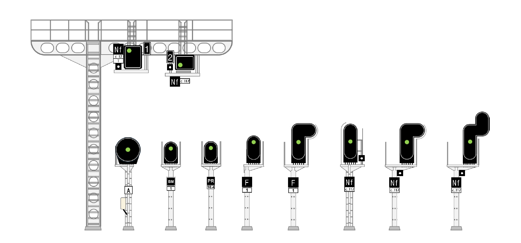
The majority of the information in this section is taken from the educational document published by the Établissement Public de Sécurité Ferroviaire (EPSF, a public institution responsible for ensuring the safety of railways in France) published on July 5, 2017.
4.2.1 - Railway risks
Not translated: please select another language
4.2.2 - Signals
Not translated: please select another language
4.2.3 - Line operation modes
Not translated: please select another language
4.2.3.1 - Single-track lines
Not translated: please select another language.
4.2.3.2 - Double-track lines
Not translated: please select another language.
4.2.4 - Train spacing systems
Not translated: please select another language
4.2.4.1 - Automatic block systems
Not translated: please select another language.
4.2.4.2 - ETCS (ERTMS)
The European Train Control System, part of ERTMS
4.2.4.2.1 - ETCS
European Train Control System
Context
The onboard computer of ETCS-enabled trains has to compute a number of position / speed curves. Here is how it works:
- below all the curves, the speed indicator is white
- above the indication curve, the speed indicator is yellow
- above the permitted curve, the speed indicator is orange
- above the warning curve, an alarm rings
- above the intervention curves, an emergency break intervention is triggered
Inputs
In order to compute any of these curves, a number of things are needed:
- target data (the destination of the braking curve, which can be EOA and SvL or LOA and MRSP)
- train data
- infrastructure data
- infrastructure manager constants
- standardized constants
Train
- max speed
- length
- rotating mass
T_traction_cutoff: the time it take to cut off traction- braking model, either lambda or gamma:
- lambda (braking weight/mass)
- gamma (constant deceleration at a given speed)
- correction factors (k_dry and k_wet for gamma braking) for braking curves
Infrastructure
- corrected gradients (it incorporates curvature)
- odometry balise locations
Processes
Braking coefficients:
A_brake_emergencyis the expected emergency braking capability, without safety marginsA_brake_safeis the emergency braking coefficient, with safety marginsA_brake_serviceis the expected service braking capability, without safety margins
Speed / distance targets
EOAend of movement authority: the location until which the train is allowed to moveSvLsupervised location: the protected location
Curves
SBDsupervised braking deceleration: intermediary result computed fromEOAandA_brake_serviceEBDemergency braking deceleration: intermediary result computed fromSvLandA_brake_safe
All the curves below are cut below a given release speed:
EBI(emergency break intervention) computed fromEBD, shifted in position and space given rolling stock metadataSBI1computed fromSBD, shifted in time withTbs1SBI2computed fromSBD, shifted in time withTbs2FLOI(also calledSBI, the intervention curve) the minimum ofSBI1andSBI2WARNING(warning curve) computed as a shift ofFLOIbyTwarningPS(permitted speed curve): shift ofWARNINGby timeTdriverINDICATIONis a shift ofPSby timeTindication
4.2.4.3 - Ks Signalling
The Ks-system (Ks = Kombinationssignal; engl: combination signal) is a german signalling system introduced in 1994 by Deutsche Bahn (DB) in order to create a common system for East Germany (Hl-System) and West Germany (H/V-System) after the german reunification.
The following paragraphs are mainly based on Pachl(2024), Railway Signalling Principles, Edition 3.0, p.20-30.
Block Section Principles
Railway lines are segmented into sequential block sections, each designed to be occupied by only one train at a time to ensure operational safety. To maintain a safe distance between two trains, the separation must account for the following components:
- the braking distance of the following train,
- the full length of the block section,
- an additional block-extension safety margin, referred to as the overlap
Block sections are delineated by main signals, which regulate train entry based on specific safety conditions. A signal may only be cleared for a train to enter a block section if all of the following criteria are met:
- the preceding train has vacated the block section in question
- the overlap beyond the next signal has also been cleared by the preceding train
- the preceding train is secured by a stop signal
- the switches for the route to be set must be locked in the correct position
- on lines with bidirectional traffic, the train must additionaly be protected against any potential opposing movements
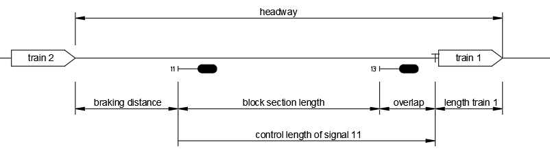
Signal control length and overlap principles
The control length of a signal refers to the section of track beyond the signal that must be verified as clear and safe before the signal can be set to proceed.
The overlap - a predefined safety margin - extends beyond the actual block section. Its primary function is to provide additional protection in the event that a train fails to stop at a signal displaying “stop”. The overlap begins at the destination signal and ends at a prominent point. Depending on the speed at which the train approaches the stop signal, different lengths of overlaps must be provided. The length of the overlap is monitored by track vacancy detection systems like axle counters.
| speed [km/h] | overlap [m] |
|---|---|
| 60 < v <= 160 | 200 |
| 40 < v <= 60 | 100 |
| v <= 40 | 50 |
A signal must remain at “stop” until the entire control length ahead is confirmed to be unobstructed. The clearing point for a signal corresponds to the end of the control length associated with the signal located behind it.
Selective Overlaps
When selective overlaps are available (only at station’s exit signals and station’s intermediate signals) different overlap options can be chosen during route setting. These alternatives may vary in length or lead into different track sections.
- An exit signal is the last signal within a station that serves to secure the exit to the free route.
- An intermediate signal is set up in extensive station areas between the entry signal and the exit signal and delimits a station section within the station.
Once the signal has been cleared, the selected overlap cannot be changed without first cancelling the route.
If a shorter-than-standard overlap is selected, the signalling system will reduce the train’s speed accordingly.
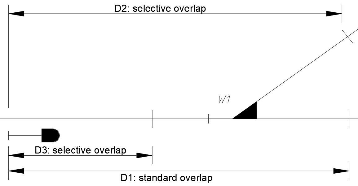
based on: DB AG, Ril 819.0202 Signale für Zug- und Rangierfahrten
Signal Indications in Ks-System
The Ks-signalling system utilizes a set of standardized signal aspects to convey operational instructions to train drivers. The primary signal indications include:
- Stop (Hp 0): The train must come to a complete stop at the signal.
- Expect stop (Ks 2): The train must be prepared to stop at the next main signal.
- Clear (Ks 1): The train is permitted to proceed.
Within the Ks-system two signalling modes are implemented:
One-Block Signalling
- The aspect displayed by a main signal is determined by the status of the immediately following block section.
- Each main signal is paired with a distant signal that provides the necessary approach indication.
- The distant signal is positioned at a distance corresponding to the braking distance from the associated main signal.
Multi-Block Signalling (Two-Block Signalling is used by DB)
- The indication of a main signal is based on the status of two consecutive block sections ahead
- This approach allows for more dynamic and anticipatory signalling, enhancing operational efficiency and safety
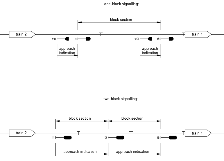
Blocking time model
To ensure undisrupted train movement, a signal must be cleared before the approaching train reaches a point where it would otherwise need to initiate braking due to the aspect of the preceding signal.
The minimum headway between two successive trains is determined by the blocking time, which defines the time interval during which a block section is exclusively reserved for a single train and thus unavailable to others.
This model is applicable not only to conventional signalling systems but also to cabin (cab) signalling systems such as LZB and ETCS.
The blocking time is composed of several distinct components:
- Signal Control Time: The time required to process and clear the signal.
- Signal Watching Time: The reaction time within which the approach signal must be cleared to prevent the driver from initiating braking.
- Approach Time: The time taken by the train to travel from the approach signal to the entrance of the block section.
- Time Between Block Signals: The duration required to traverse the distance between consecutive block signals.
- Clearing Time: The time needed for the train to fully vacate the block section, including the overlap.
- Release Time: The time required to unlock and release the block section for use by subsequent trains.
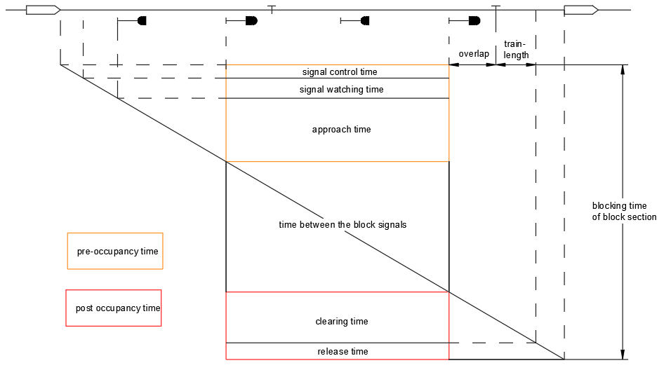
Appearance of Ks-Signals with speed indicators
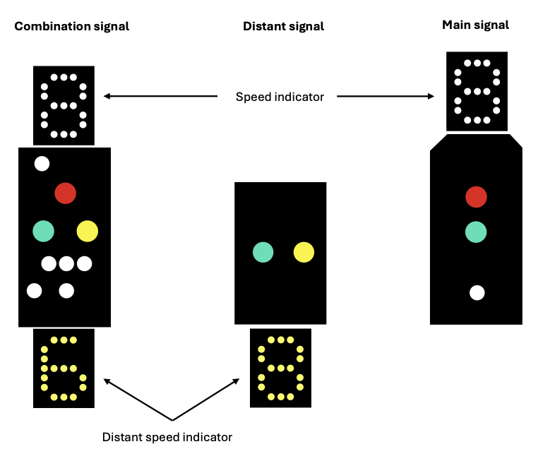
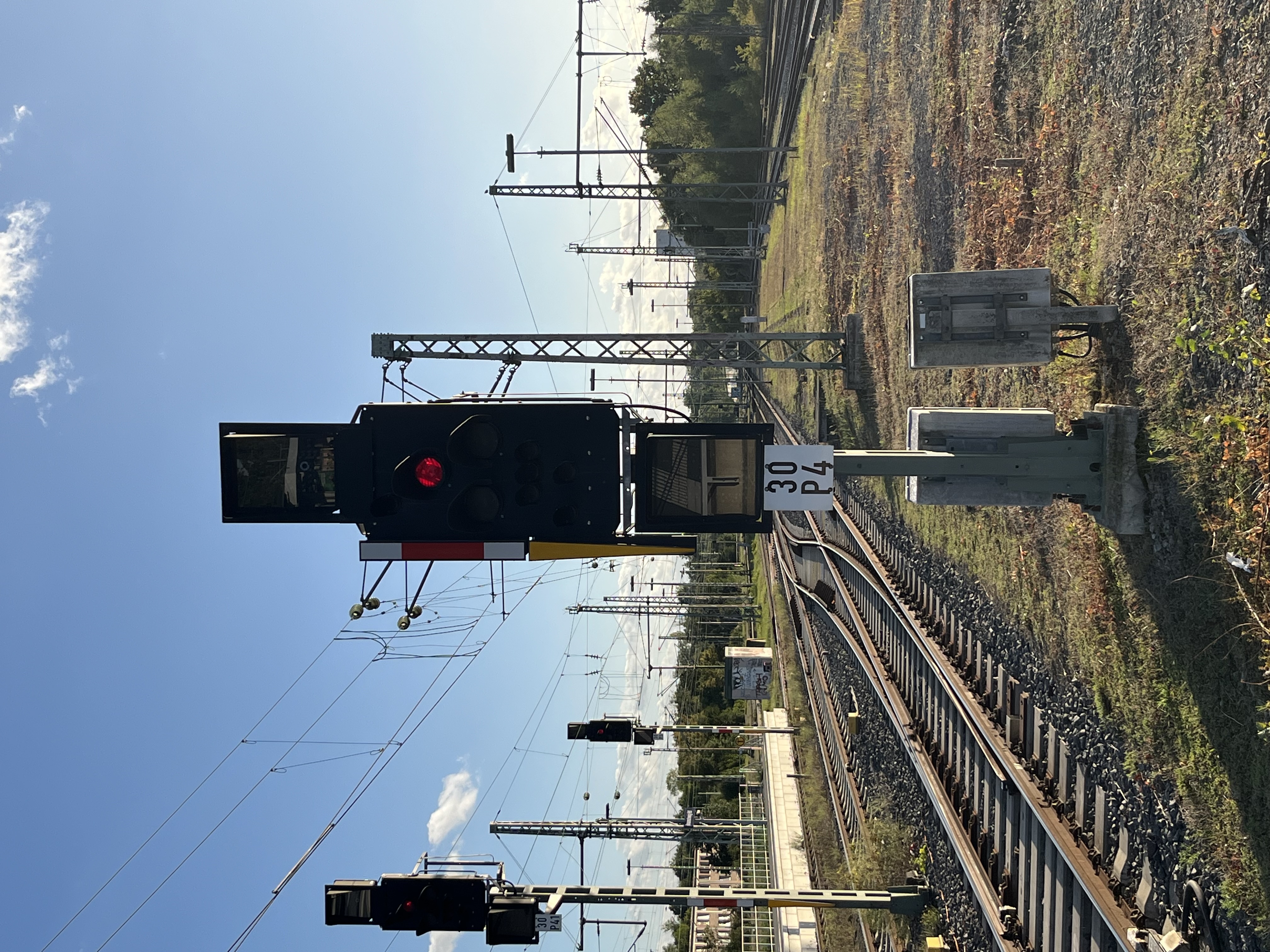
Ks-signal in Braunschweig main station, Source: Dominik Wefering
Signal Indications on a Ks-Signal
| Description | Aspect | Meaning |
|---|---|---|
| Combination signal | 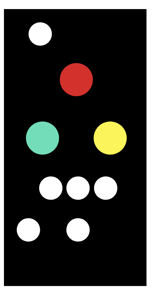 | combination signals have the function of both main signal and distant signal |
| main signal | 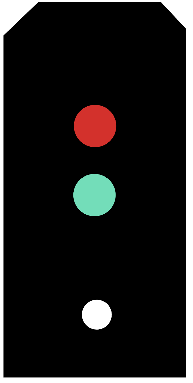 | main signals indicate whether the track section ahead may be run over |
| distant signal |  | Distant signals indicate which signal aspect is to be expected at the corresponding next main signal.These are positioned at the braking distance from the next main signal |
| Stop (Hp 0) |  | the signal prohibits the passing of a train |
| Clear (Ks 1) |  | 1. The signal permits the passing at the maximum speed allowed on the section, unless a speed restriction is indicated by a speed indicator.2. The green luminous spot blinks if a distant speed indicator shows in the signal, indicating a speed restriction at the next main signal |
| Expect Stop (Ks 2) |  | the signal permits the passing and indicates a stop at the next main signal |
based on: Bailey(1995), European Railway Signalling, p58; sprites from https://github.com/Nakaner/railway-signals.git
Speed Indicators in the Ks-Signalling System
The Ks system includes specific indicators to communicate speed restrictions to train drivers.
Speed Indicator (Zs 3)
- The speed displayed by the Zs 3 indicator defines the maximum permissible speed from the signal onward, specifically within the subsequent switch area.
- The numeric value shown on the indicator represents the allowed speed in kilometers per hour, calculated as 10 times the displayed number.
Distant Speed Indicator (Zs 3v)
- means: expect speed indicator Zs 3
- The Zs 3v indicator provides advance notice of a speed restriction at the next main signal.
- Similar to the Zs 3 indicator, the displayed number corresponds to a permissible speed of 10 times the value in km/h at the upcoming main signal.
Source: DB AG, Ril 301 Signalbuch
| Aspect | Form | Light | Corresponding speed-limit |
|---|---|---|---|
| Zs 3 |  |  | 80 km/h from this signal |
| Zs 3v | 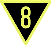 |  | 80 km/h from the corresponding main signal |
sprites from https://github.com/Nakaner/railway-signals.git
4.2.4.3.1 - Linienförmige Zugbeeinflussung (LZB)
Overview
The Linienförmige Zugbeeinflussung (LZB) is a continuous automatic train control system used to ensure safe and efficient operation at high speeds. Unlike the Punktförmige Zugbeeinflussung (PZB) (see PZB), which transmits discrete signal information at fixed track points, the LZB enables continuous bi-directional data exchange between the train and the trackside control center. This allows for real-time supervision of speed and position and forms the basis for cabin signalling at speeds exceeding 160 km/h.
System Structure
The LZB consists of three main components (DB, 2019):
Trackside Equipment
The track contains cable loops laid between the rails, divided into multiple segments.
These loops enable continuous communication between the train and the LZB control center.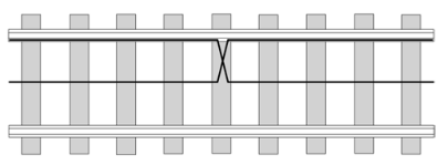
Source: Pachl (2022)
Train Equipment
Each LZB-equipped vehicle has an onboard unit that:- continuously determines the train’s position,
- receives and interprets control information from the LZB center,
- calculates braking curves and speed supervision data,
- and automatically applies braking if limits are exceeded.
LZB Control Center
The control center transmits Movement Authorities (MAs) to the trains within the controlled area, defining:- the permissible target distance,
- the permitted speed at each section,
- and other route-specific properties like gradients
Functionality
During operation, the train continuously reports its position to the LZB center. In return, it receives updated target data like setpoint speed (\(v_{set}\)), target speed (\(v_{target}\)) and target distance.
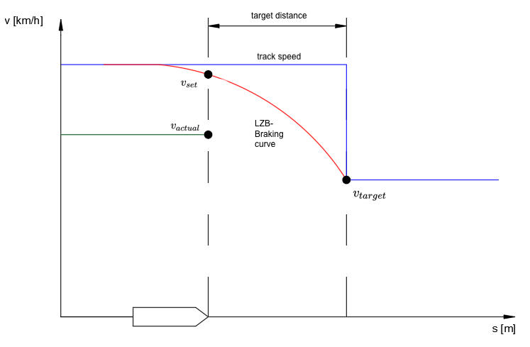
based on: Pachl (2022)
The onboard unit calculates braking curves for different supervision thresholds:
- Permitted Speed Curve – permissible maximum speed at each position. This is the curve the driver train should follow.
- Warning Curve - gives an acoustic warning to the driver when the permitted speed curve is exceeded by 5 km/h.
- Emergency Brake Curve – triggers an emergency brake if the train fails to decelerate sufficiently.
The braking curve that is set by the onboard unit is based on:
- maximum track speed
- slope¹
- braking percentage of the train
The next target point is displayed up to 10.000 m in front of the train. The speed limit equals the maximum track speed or the maximum possible speed of the train itself. (Murr, 1991)
Braking Curves
For LZB there exist twelve braking curves with values between 0,115 und 1,10 m/s². The value of the emergency braking curve is about 40% higher than the permitted speed curve.
The deceleration of the individual braking curves remains constant across the entire speed range.
| Braking Curve Nr (BRN) | A | B | 1 | 2 | 3 | 4 | 5 | 6 | 7 | 8 | 9 | 10 |
|---|---|---|---|---|---|---|---|---|---|---|---|---|
| Emergency Braking Curve [m/s²] | 0,115 | 0,2 | 0,29 | 0,375 | 0,460 | 0,545 | 0,63 | 0,715 | 0,8 | 0,9 | 1,0 | 1,1 |
| Permitted Speed Curve [m/s²] | 0,08 | 0,14 | 0,21 | 0,27 | 0,33 | 0,39 | 0,45 | 0,51 | 0,57 | 0,64 | 0,71 | 0,79 |
based on: Braun (1988)
The illustration below shows the braking curves for BRN 6 as an example.
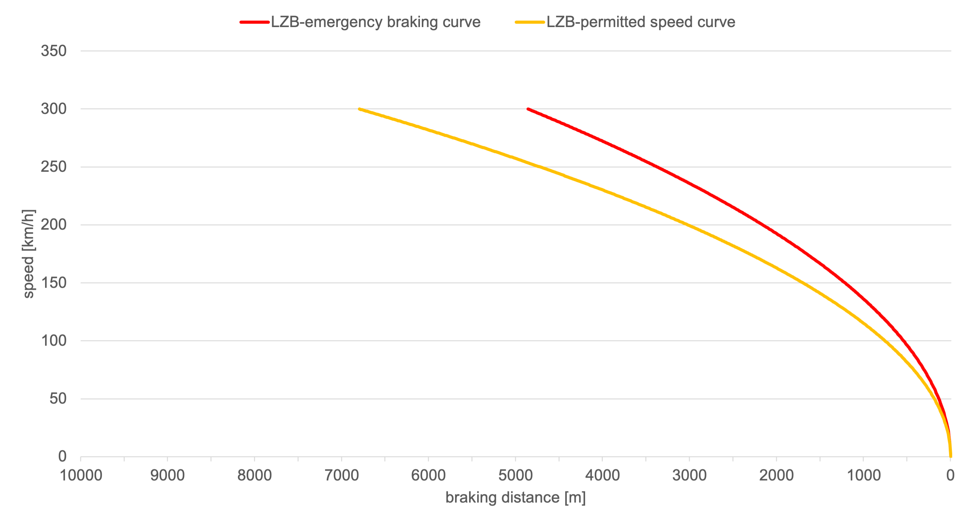
The train driver enters the permissible speed and the brake percentage into the vehicle device. The gradient is specified for the route. The LZB uses this data to set the necessary braking curve. (Braun, 1988)
For Passenger trains the following curves must be set:
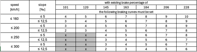
based on: Braun (1988)
For freight trains the following curves must be set:
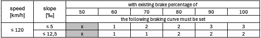
based on: Braun (1991)
Where an “x” is written the combination of braking percentage and speed must not be possible.
Full Block and Partial Block Mode
The LZB can operate in two different control modes: Full Block Mode (german: Ganzblockmodus) and Partial Block Mode (german: Teilblockmodus). Both modes determine how the track is divided into supervised sections and how the control center grants Movement Authorities (MAs) to trains.
In Full Block Mode, each train occupies an entire block section, similar to traditional fixed-block signalling systems. A new train is only allowed to enter a block once the preceding train has completely cleared it. This mode ensures maximum safety but limits the line capacity. (Pachl, 2022)
In Partial Block Mode, the LZB subdivides a block into several smaller LZB subsections. Each subsection can be individually monitored and released as the train progresses, allowing the following train to enter the same block earlier. This dynamic release mechanism increases line capacity significantly while maintaining safe separation between trains. (Pachl, 2022) The partial block principle thus enables higher traffic density and shorter headways, which are especially important for high-speed or high-frequency railway operations. The typical length of a LZB subsection is about 1200 m (Busse, 2021)
The picture below shows the Partial Block Mode. Train 1 occupies the block between the two main signals. Train 2 is a LZB train and is therefore allowed to enter the block until the section marker. Train 3 is not equipped with LZB and is therefore not allowed to enter the occupied block.
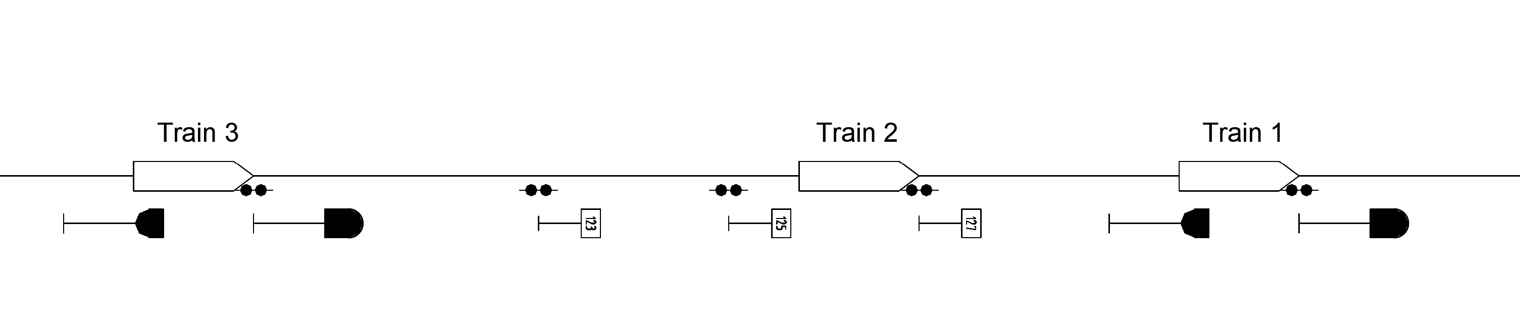
OSRD-modeling
Braking curve is based on the permitted speed curve.
Warning curve and emergency braking curve are not modeled.
The braking curve is constant over the whole braking distance.
The constant deceleration is used for braking to a full stop, for speed changes and for the spacing and routing requirements.
For Partial Block Mode, LZB section markers are placed at the entry of LZB subsections.
Switches are released when the following detector is crossed.
There are no overlaps implemented yet (only affects blocking time).
Simplifications and Assumptions
All LZB-trains have a sight distance of 10.000 m (impacts the distance for average slope calculation, and maybe future work on dynamic simulation).
The slope used to choose the braking curve is the average slope calculated within these 10.000 m.
The train follows the permitted speed curve and does not brake earlier.
OSRD trains do not have brake percentage values, so an alternative to define the used braking curves was used:
- The braking curves are picked depending on the rolling stock category, the train’s maximum speed and the average slope (exact modeling and code to be determined).
Determination of the braking curve
The average deceleration of each speed category was calculated and the corresponding braking curves were chosen. The resulting curves are also the ones that are used the most.
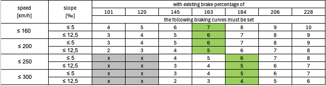
The resulting curves for ≤ 200 and ≤ 250 km/h were the same so they were put together in one category
This results in the following braking curves that must be set for passenger trains:
Slope [‰] ≤ 160 km/h 160 - 250 km/h 250 - 300 km/h ≤ 5 7 6 5 ≤ 12,5 6 5 4 The corresponding deceleration (permitted speed curve) values that must be set for passenger trains depending on the maximum train speed and slope are as follows:
Slope [‰] ≤ 160 km/h 160 - 250 km/h 250 - 300 km/h ≤ 5 0,57 0,51 0,45 ≤ 12,5 0,51 0,45 0,39 possible further simplification for OSRD: deceleration in other LZB-modeling tools is 0,5 for all passenger trains
For freight trains only two decelerations (permitted speed curve) were chosen. They cover all the relevant cases for freight trains with LZB.
Slope [‰] ≤ 120 km/h ≤ 5 0,33 ≤ 12,5 0,27 possible further simplification for OSRD: deceleration in other LZB-modeling tools is 0,3 for all freight trains
References
- Alfred Braun. „Aufstellen von Bremstafeln für Strecken mit Linienzugbeeinflussung“. In: ZEV Glasers Annalen 4 (1988), S. 108–118.
- Alfred Braun. “Die LZB-Bremstafeln für Güterzüge”. In: Eisenbahningenieurkalender (1991), S. 275-282
- DB AG. Ril 819.1320 LZB; Grundsätze für die Ausrüstung mit linienförmiger Zugbeeinflussung. Dez. 2019.
- Eduard Murr. „Systembeschreibung der Linienzugbeeinflussung (LZB) der Deutschen Bundesbahn“. In: Eisenbahningenieurkalender (1991), S. 285–317.
- Jörn Pachl. Systemtechnik des Schienenverkehrs: Bahnbetrieb planen, steuern und sichern. de. Wiesbaden: Springer Fachmedien Wiesbaden, 2022.
- Matthias Busse. „Der optimierte Einsatz von ETCS-Bremskurven“. Dissertation. Dresden: Technische Universität Dresden, Feb. 2021.
¹ The slope is saved in the LZB-Control Center. We don’t yet have reliable information on how the slope in front of the train is calculated, when determining the braking curve.
4.2.4.3.2 - Punktförmige Zugbeeinflussung (PZB)
Overview
The Punktförmige Zugbeeinflussung (PZB) is an intermittent train protection system used on most conventional railway lines in Germany.
Its primary function is to ensure that trains respond correctly to restrictive signal aspects and speed limits.
The PZB monitors the train’s compliance with braking requirements and automatically initiates braking interventions when these are violated.
The system acts as a safeguard against driver inattention or failure to observe signals and thereby prevents trains from passing stop signals or exceeding permitted speeds (DB, 2014).
The core tasks consist of monitoring braking maneuvers, protecting against trains continuing past stop signals, and preventing trains from moving forward against stop signals, for example after a scheduled stop at platform (DB, 2024).
System Components
The PZB consists of two main parts:
- Trackside equipment, composed of inductive magnets installed along the track near signals.
- Onboard equipment, located on the locomotive to communicate with the magnets and supervise train operation.
Trackside Magnets
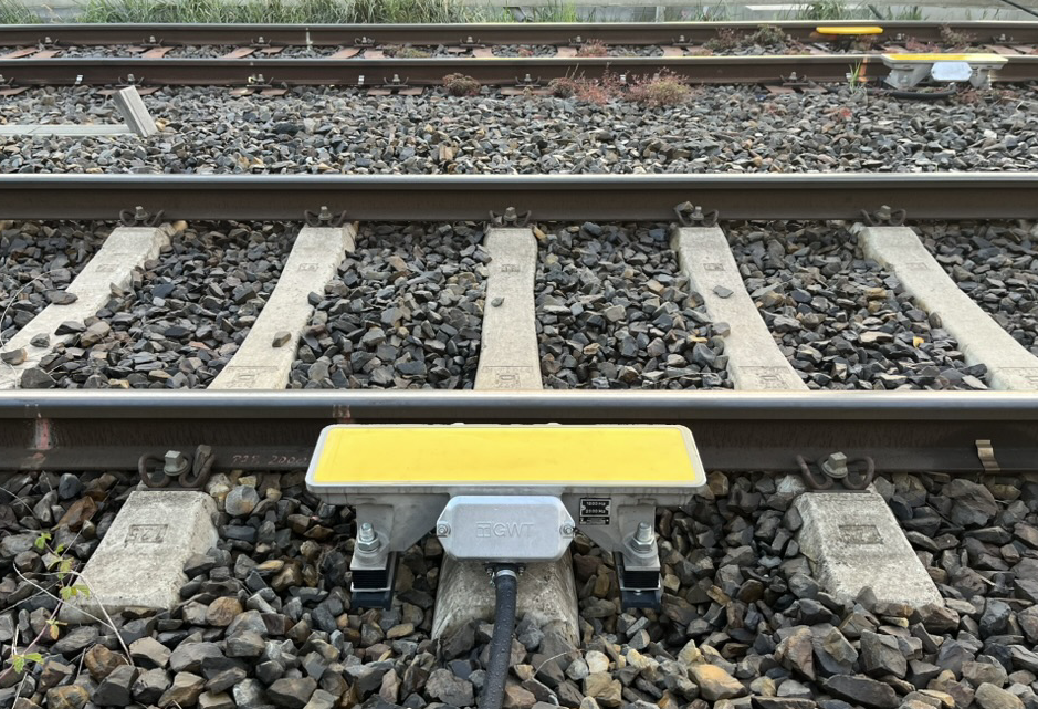
Source: Dominik Wefering
Three types of track magnets are used, each operating at a distinct frequency (DB, 2014):
| Frequency | Location | Function |
|---|---|---|
| 1000 Hz | At the distant signal | Activates supervision when the distant signal shows a restrictive aspect (Ks 2). The driver must acknowledge the magnet within 2,5 seconds and a braking sequence begins. |
| 500 Hz | About 260 m before the main signal | Reinforces braking supervision before a stop signal. The train must reduce its speed further. |
| 2000 Hz | At the main signal | Immediately triggers an emergency brake if the train passes a stop signal (Hp 0). |
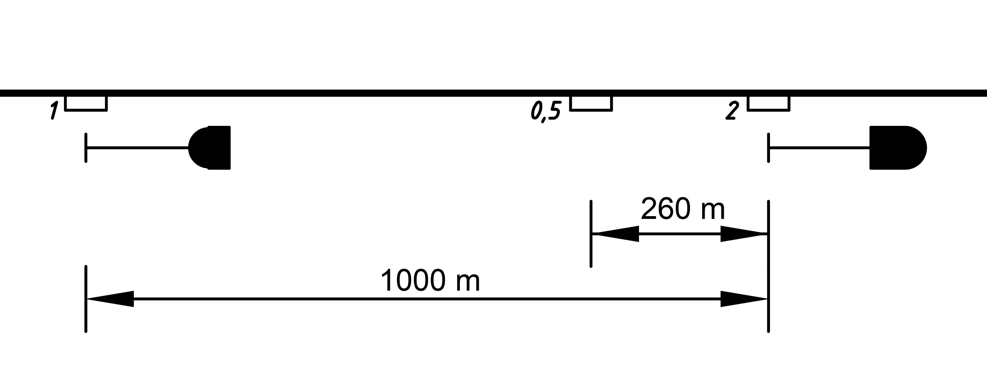
On combination signals (see Ks Signalling) there are double-track magnets with frequencies of 1000 and 2000 Hz combined.
The picture below shows an distant signal with the aspect Ks 2 and the 1000 Hz magnet to the left of the signal.
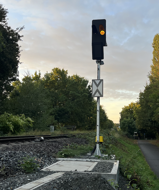
Source: Dominik Wefering
Onboard Equipment
The onboard system receives inductive signals from the track magnets and monitors (DB, 2014):
- The acknowledgement of signal aspects by the driver.
- The elapsed time and distance since the last magnet activation.
- The train speed relative to permitted limits defined by the current supervision state.
If the driver fails to acknowledge or reduce speed as required, the system triggers an automatic emergency brake until a full stop.
Train types
PZB makes a distinction between three train types (german: Zugart): O, M, U
- O = Upper train type (german: Obere Zugart)
- M = Middle train type (german: Mittlere Zugart)
- U = Lower train type (german: Untere Zugart)
The distinction is based on the brake percentages of the train (Maschek, 2022):
| Train type | Brake percentages | monitored maximum speed |
|---|---|---|
| O | > 110 | 165 |
| M | 66 - 110 | 125 |
| U | < 66 | 105 |
The braking percentage is a standardized measure in railway operations used to quantify a train’s braking capability.
It is defined as the ratio of the effective braking weight (B) to the train mass (m), multiplied by 100 (Kache, 2024):
$$ \lambda=\frac{B}{m}*100 $$
This value indicates how effectively a train can decelerate relative to its mass. A higher braking percentage corresponds to a shorter braking distance, allowing for a direct comparison between different trains.
Supervision Logic of PZB
The system evaluates train movement against predefined supervision limits. Each magnet initiates a specific monitoring function:
- Time-based supervision
- Distance-based supervision
- Speed thresholds
These parameters are dynamically managed depending on the train type.
Basic principle of PZB supervision
The basic principle of the supervision curves in PZB is shown in the following illustration (see following schema for the exact shape of decrease):
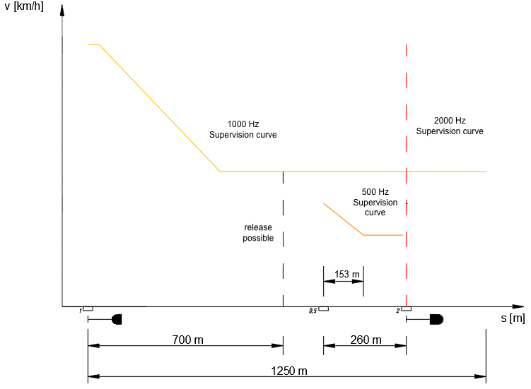
based on Maschek (2022)
Supervision Curves
The supervised values depending on the train type are as follows:
| Train type | Upper (O) | Middle (M) | Lower (U) |
|---|---|---|---|
| Maximum Speed | 165 km/h | 125 km/h | 105 km/h |
| Braking curve of 1000 Hz influence | 85 km/h after 23 Sec. | 70 km/h after 29 Sec. | 55 km/h after 35 Sec. |
| Braking curve of 500 Hz influence | from 65 to 45 km/h within 153 m | from 50 to 35 km/h within 153 m | from 40 to 25 km/h within 153 m |
The values in the table above result in the following six supervision curves for the PZB for each train type:
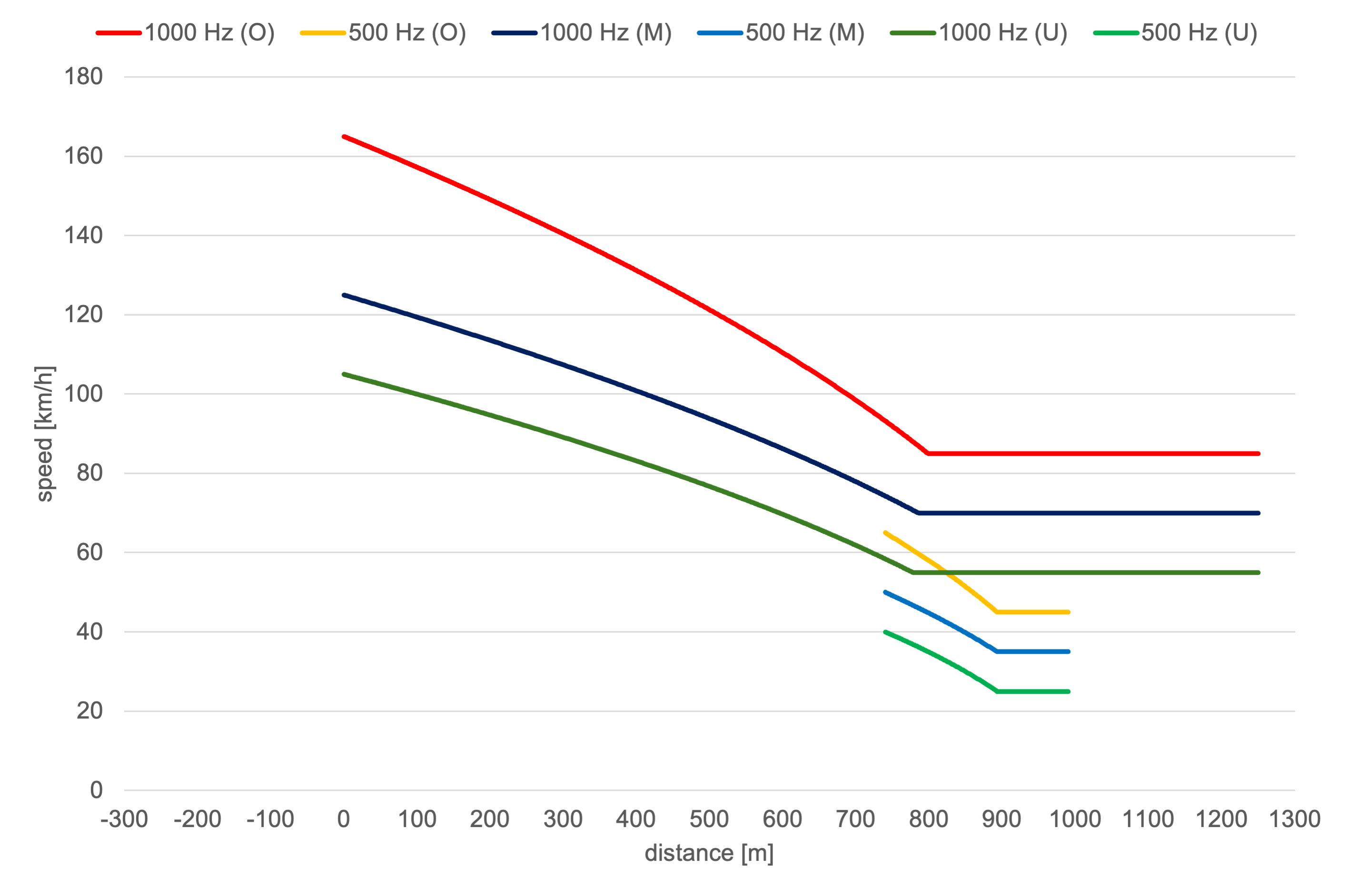
Release from 1000 Hz supervision
700 m after the 1000 Hz influence, the train driver can stop braking if the main signal has turned back to Ks 1 in the meantime. In this case, he can accelerate again to the maximum permitted speed.
Restrictive Mode
If a train stops while a PZB supervision is active, or if its speed drops below the switching speed of 10 km/h for at least 15 seconds, more restrictive supervision curves are activated.
In this restrictive mode, the 1000 Hz supervision curve is lowered to a maximum permissible speed of 45 km/h.
Similarly, for the 500 Hz supervision, the system enters a restrictive state if, within the 153 m monitoring section, the train travels for more than 15 seconds below the switching speed of 30 km/h, while the speed continues to decrease toward 10 km/h.
Typical example: When a train stops at the platform, the overlap behind the destination signal is cleared and the switches are released. The restrictive curves ensure that if the train starts moving without permission after stopping, it will travel slowly enough so as not to pose a danger to other trains. Once it arrives at the 2000 Hz magnet, its speed will be low enough for the emergency brake to make it come to a full stop wihtin the overlap.
Safety Function
The PZB ensures safety through automatic emergency braking when:
- The driver fails to acknowledge a restrictive signal,
- The train exceeds the monitored speed during supervision,
- Or a stop signal (Hp0) is passed.
This guarantees that even under human error or distraction, train operations remain within safe limits and the risk of signal overruns is minimized.
OSRD-modeling
The supervision curves are only used for calculating the deceleration values. They are not modeled in OSRD.
Emergency braking is not modeled and restrictive mode is not modeled.
The PZB braking curve is modeled for each train type with two constant decelerations \(a_{type,1}\) and \(a_{type,0,5}\).
The deceleration is used for braking to a full stop, for slowdowns and for spacing and routing requirements.
\(a_{type,1}\) corresponds to a deceleration that brakes the train from the maximum speed applicable to the train type \(v_{type,max}\) down to below the check speed of the 500 Hz condition \(v_{type,check,0,5}\) (1000 Hz phase).
\(a_{type,0,5}\) corresponds to a deceleration that brakes the train from the speed below the check speed \(v_{type,res,0,5}\) to a full stop within the distance between the 500 Hz Magnet and the associated main signal (500 Hz phase).
There are no overlaps implemented yet (only affects blocking time).
As PZB trains can use LZB tracks, in addition to LZB signal data should provide PZB signal at the entry of the LZB block and not at the entry of LZB subsections (It is only used for LZB partial block mode).
Simplifications and assumptions
There is no infrastructure model for magnets in OSRD. The modeling is therefore based on signal locations.
A constant distance of \(s_{0,5}\) = 260 m is assumed as fictitious trigger of the 500 Hz phase.
A distant signal spacing of \(s_{distant}\) = 1000 m is assumed.
A sighting distance for distant signal of \(s_{sight}\) = 300 m is assumed.
OSRD trains do not have brake percentage values, so an alternative to define the used braking curves was used:
The braking curves are set depending on the rolling stock category and the train’s maximum speed.
- Upper Train type: Passenger Train with \(v_{O,max}\) = 165 km/h,
- Middle Train type: Freight or Passenger Train with \(v_{M,max}\) = 125 km/h,
- Lower Train type: Freight train with \(v_{U,max}\) = 105 km/h.
Calculating the deceleration values
At first we have to calculate the deceleration for the 1000 Hz Phase, which was done with:
$$ a_{type,1}=\frac{v²_{type,max}-v²_{type,check,0,5}}{2*(s_{sight}+s_{distant}-s_{0,5})} $$
| Value | Meaning |
|---|---|
| \(a_{type,1}\) | Deceleration of the 1000 Hz phase |
| \(v_{type,max}\) | Maxmimum speed per train type |
| \(v_{type,check,0,5}\) | Check speed of 500 Hz Magnet per train type |
| \(s_{sight}\) | Sighting distance for distant signals |
| \(s_{distant}\) | Distant signal distance |
| \(s_{0,5}\) | Distance of 500 Hz magnet from main signal |
The result was rounded up to two decimal places to have a fixed value and a small margin for the actual speed-check of the 500 Hz magnet.
Then with this deceleration the resulting speed at the position of the 500 Hz magnet \(v_{type,res,0,5}\) was calulated.
The next step was calculating the deceleration value for the 500 Hz phase:
$$ a_{type,0,5}=\frac{v²_{type,res,0,5}}{2*s_{0,5}} $$
| Value | Meaning |
|---|---|
| \(a_{type,0,5}\) | Deceleration of the 500 Hz phase |
| \(v_{type,res,0,5}\) | Resulting speed after 1000 Hz phase |
Stop braking curve
The resulting braking curves for each train type are as follows:
The 1000 Hz and 500 Hz curves are displayed for informational purpose only.
- Upper train type (O)
- \(a_{O,1}\) = 0,86 m/s² for the 1000 Hz phase and
- \(a_{O,0,5}\) = 0,6 m/s² for the 500 Hz phase.
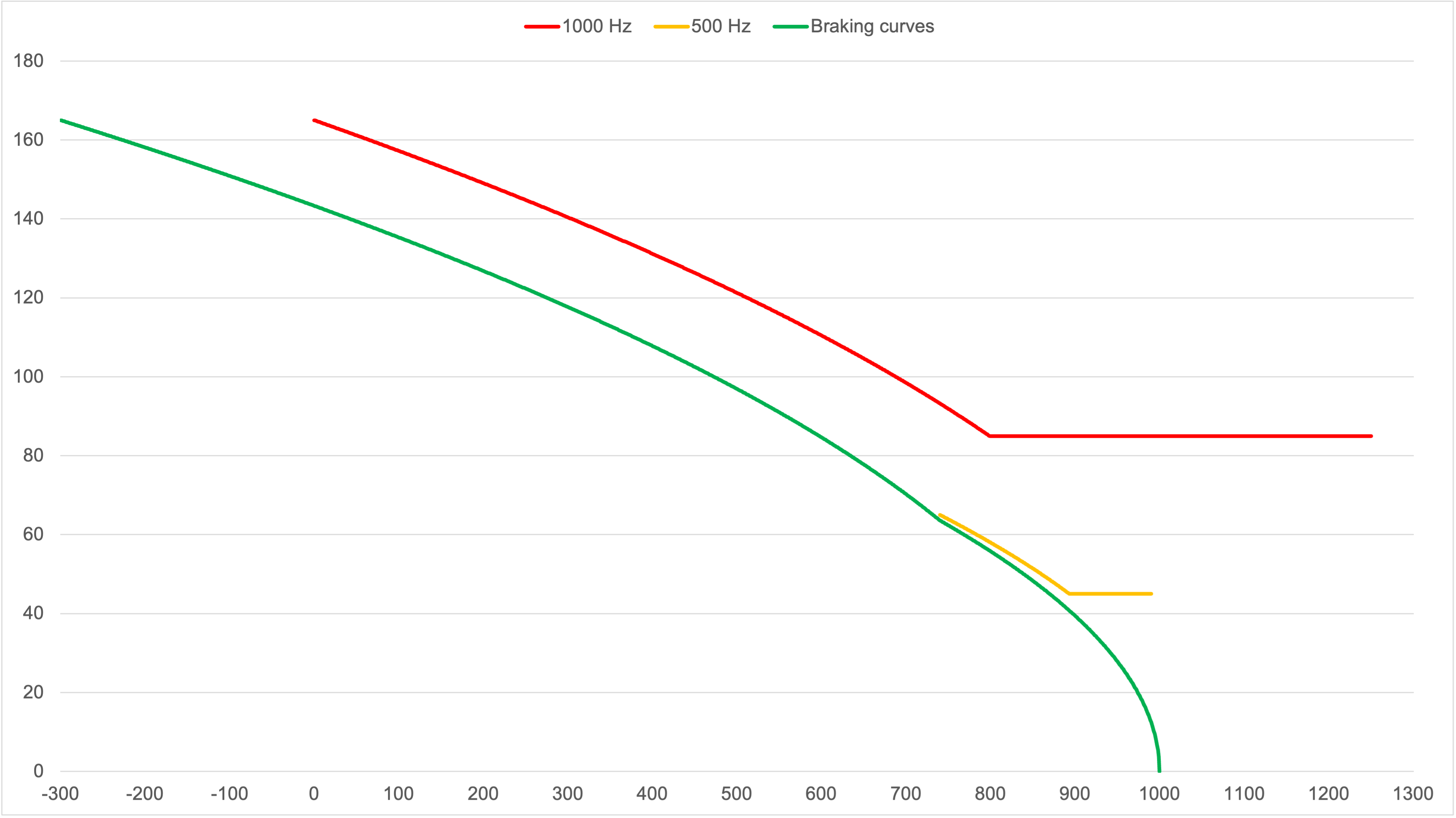
- Middle train type (M)
- \(a_{M,1}\) = 0,49 m/s² for the 1000 Hz phase and
- \(a_{M,0,5}\) = 0,36 m/s² for the 500 Hz phase.
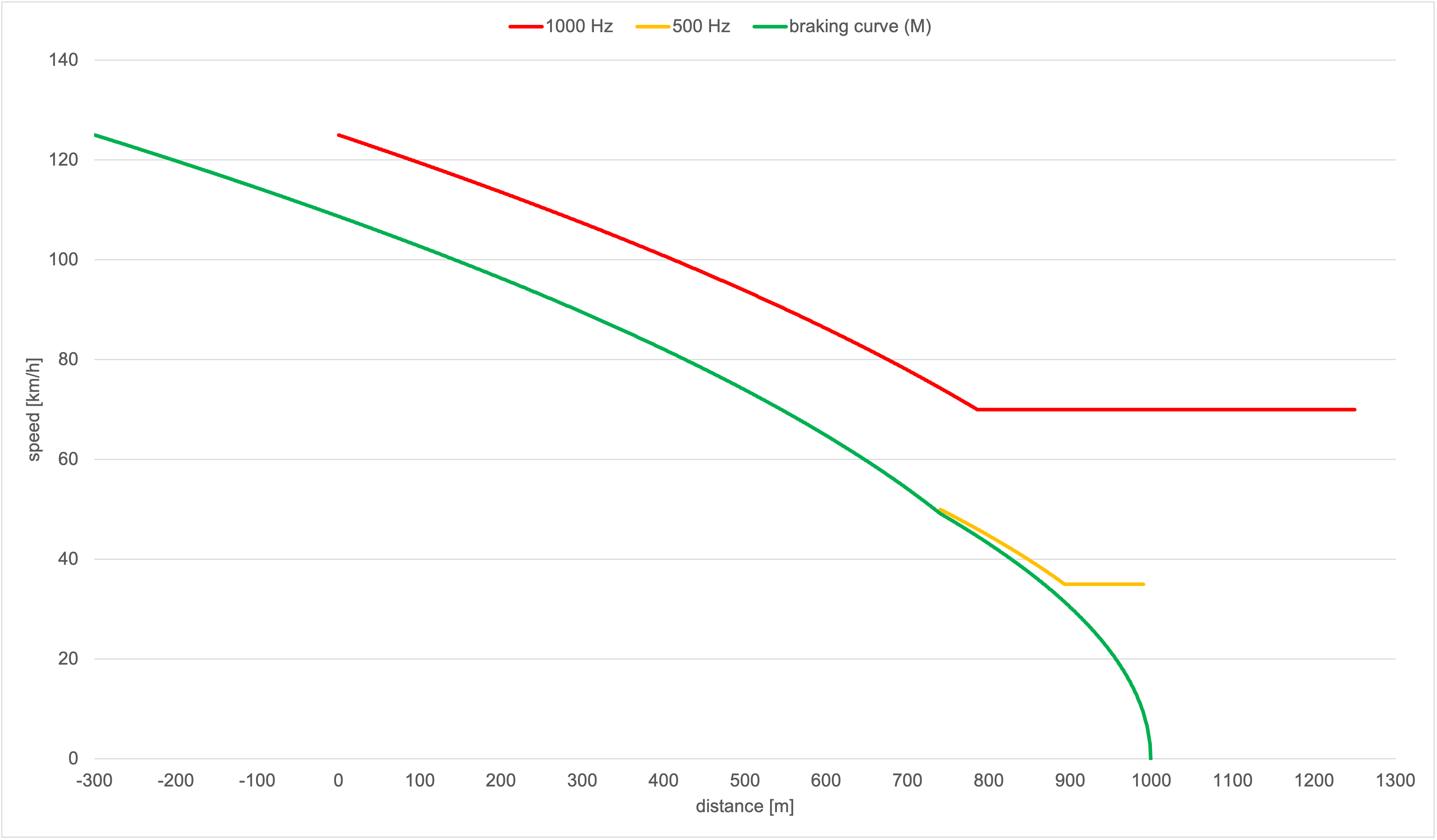
- Lower train type (U)
- \(a_{U,1}\) = 0,36 m/s² for the 1000 Hz phase and
- \(a_{U,0,5}\) = 0,2 m/s² for the 500 Hz phase.
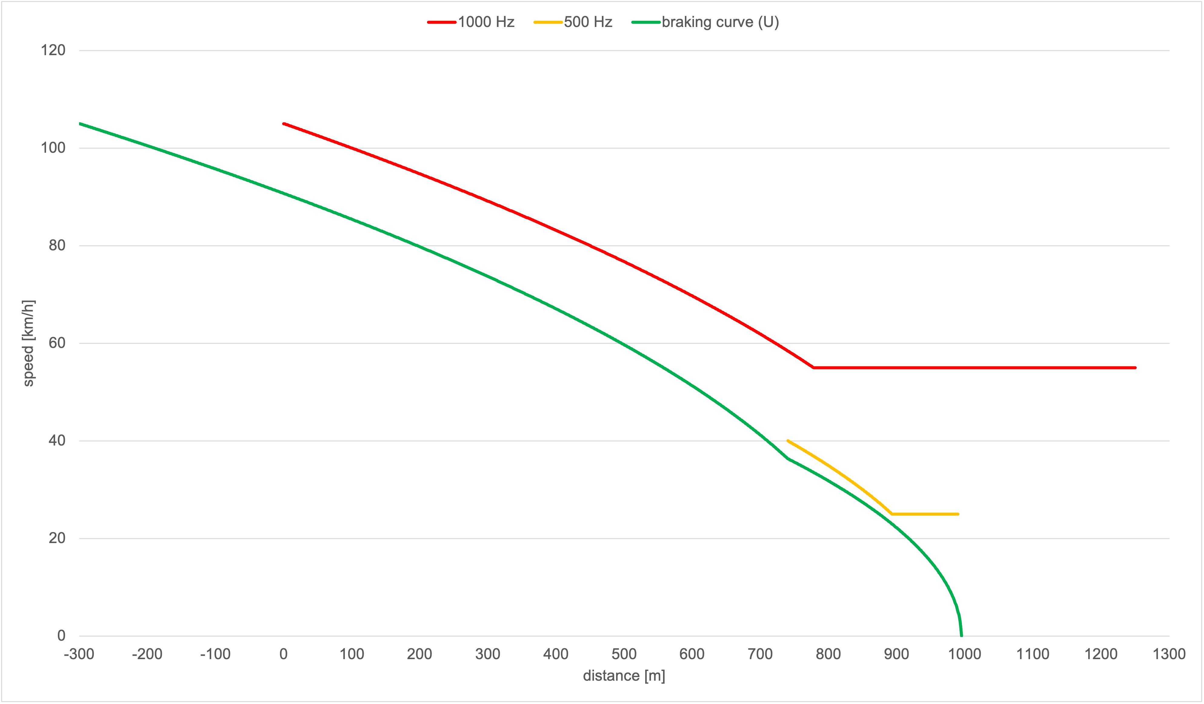
Slowdown braking curve
In lineside signalling like the Ks Signalling the speed restrictions generally apply at the next main signal. Therefore the slowdown needs to be handled differently, otherwise a train could harm the PZB conditions if the braking curve is applied to the destination point with the speed restriction.
For slowdowns there are two cases:
The target speed is equal or higher than the initial checked speed of the 500 Hz magnet: The train brakes directly to the destination with the constant deceleration of \(a_{type,1}\). This allows to save some capacity, since the train is able to brake later.
The target speed is below the initial checked speed of the 500 Hz magnet: The train follows the stop braking curve until it reaches the target speed and then the train continues in a steady-state running at the target speed (release speed).
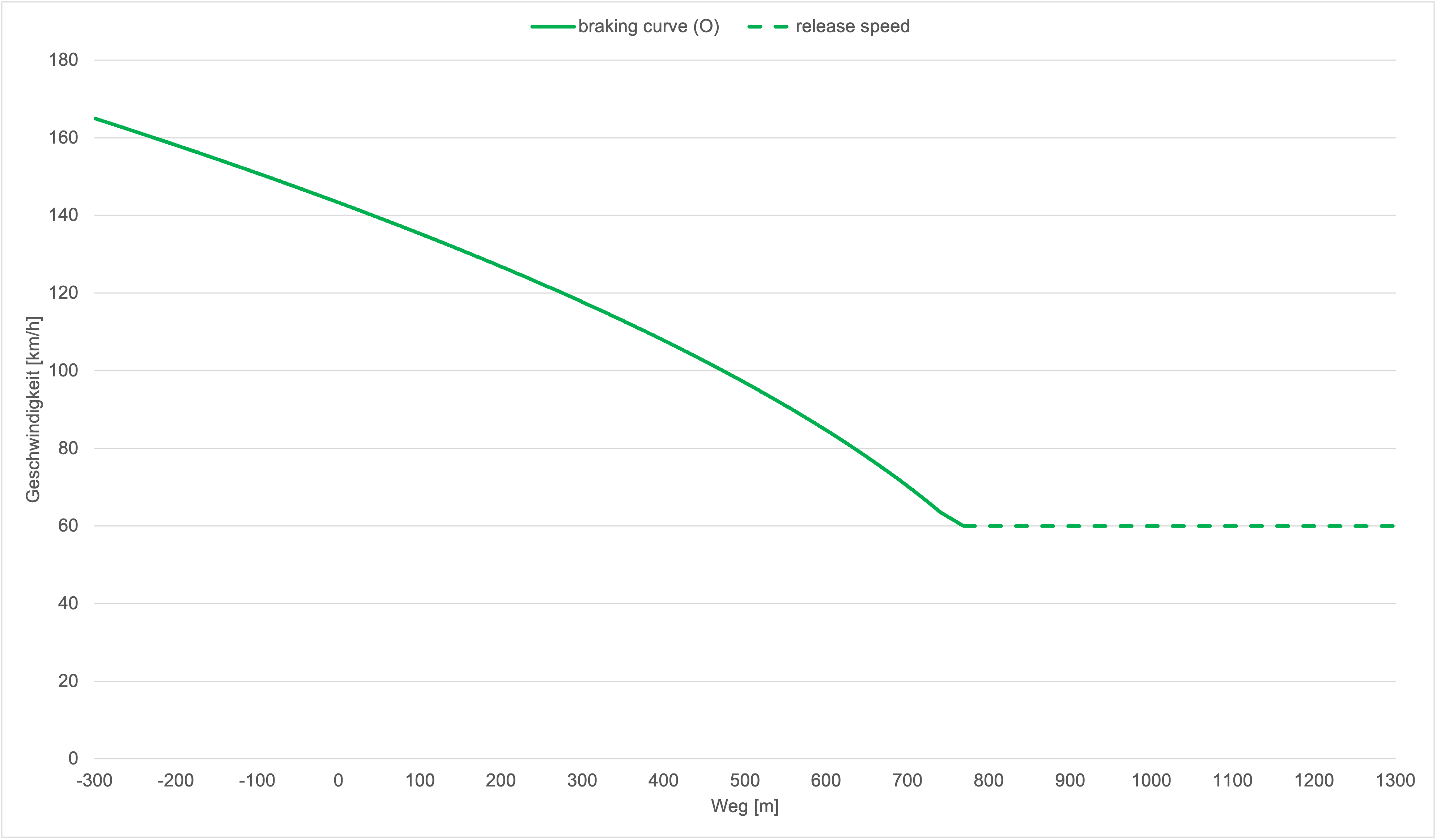
References
- DB AG. Ril 483.0111 Punktförmige Zugbeeinflussunganlagen bedienen. Aug. 2014
- DB AG. Ril 819.1310 Punktförmige Zugbeeinflussung (PZB); Grundsätze für das Ausrüsten von Strecken. Juli 2024.
- Martin Kache. Fahrdynamik der Schienenfahrzeuge: Grundlagen der Leistungsauslegung sowie der Energiebedarfs- und Fahrzeitberechnung. de. Wiesbaden: Springer Fachmedien Wiesbaden, 2024
- Ulrich Maschek. Sicherung des Schienenverkehrs: Grundlagen und Planung der Leit- und Sicherungstechnik. de. Wiesbaden: Springer Fachmedien Wiesbaden, 2022.